Data Sources and Variables |
||
Variable |
Measure |
Source |
|---|---|---|
Outcome variable - from Prison Policy Initiative |
||
| Rate of imprisonment | per 100,000 residents | Prison Policy Initiative |
Established indicators (demographics and socioeconomic) - from US Census |
||
| Black residents | percent | US Census Data |
| Median income | in thousands | US Census Data |
| Unemployment rate | percent | US Census Data |
| Urban/Rural Classification | dummy | US Census Data |
Primary explanatory variables - from SAMHSA |
||
| Travel time to mental health facility | minutes at 9:00 am on a weekday from the center of the tract | Substance Abuse and Mental Health Services Administration |
| Distance to mental health facility | driving miles from the center of the tract | Substance Abuse and Mental Health Services Administration |
| Travel time to inpatient facility | minutes at 9:00 am on a weekday from the center of the tract | Substance Abuse and Mental Health Services Administration |
| Driving miles to inpatient facility | driving miles from the center of the tract | Substance Abuse and Mental Health Services Administration |
| Travel time to inpatient facility w/ crisis intervention | minutes at 9:00 am on a weekday from the center of the tract | Substance Abuse and Mental Health Services Administration |
| Driving miles to inpatient facility w/ crisis intervention | driving miles from the center of the tract | Substance Abuse and Mental Health Services Administration |
Reference Data - from American Community Survey |
||
| Tract shapfiles | geometric vector | American Community Survey |
Introduction
In 2022, the federal, state, and local governments of the United States held almost two million people in some form of detention in over 6,300 facilities (Sawyer & Wagner, 2023). The systems that contribute to this large number of incarcerated people in the US have been growing steadily over the past half-century. In 1998, activist and former political prisoner Angela Davis was the first to use the term “prison industrial complex” to refer to the massive industrialized profit-driven systems that make up the penal system in the US. She said the “prison industrial system materially and morally impoverishes its inhabitants and devours the social wealth needed to address the very problems that have led to spiraling numbers of prisoners” (Davis, 1998).
As the Prison Industrial Complex (PIC) has expanded, scholars have examined the relationship between place and imprisonment in terms of places with high rates of reported crime, places with an overwhelming police presence, and the experiences of people in those communities and their relationship with the criminal justice system. The removal of individuals from an already struggling community only contributes to the cycle of instability that leads to crime and harm. These individuals are fathers, workers, caregivers, and other valuable members of their community; ripping them from their families not only impacts those who may have violated the law but also those they leave behind who may have been financially or emotionally dependent on them (Gilmore, 2007).
A number of alternative measures have been proposed against mass incarceration, including the legalization of marijuana, the repeal of discriminatory “tough on crime” laws, and drug courts and other treatment programs (Braun, 2019; Porter, 2022). This research focuses on a different approach to the problem of mass incarceration—access to mental health, specifically inpatient care and crisis intervention. While this may not be a fully causal analysis, the association between access to mental health care and imprisonment rates combined with medical research about violent behavior and mental health care may provide insights about potential areas in need of these types of resources.
Any analysis of the PIC should include an examination of the demographic and socioeconomic factors associated with high imprisonment rates, and this analysis is no exception. The analysis of these relationships provides context about the harm caused by the PIC and that harm may be compounded by issues of access to mental health care and its relationship with imprisonment rates. In this evaluation, I focus on place-based implications of access to mental health care and imprisonment using only one dimension of access—proximity in travel time or miles. (It is worth noting here that the intention was to include the capacity of the nearest facility as it is related to population density in addition to proximity, but due to the fact that none of the facilities contacted for this project would provide any information about capacity or any other details about the care they provide, this analysis is limited to only distance.) By exploring the proximity of care and the characteristics of census tracts, this research may illuminate insights about areas in need of more resources for mental health accessibility to improve outcomes for communities overly impacted by an oppressive carceral system. Considering these spatial characteristics along with standard factors and existing research may illuminate an unexplored piece of the greater influence of oppressive policies that fuel the prison industrial complex as a whole.
Literature Review
It has been well documented that people of color, especially Black men, are more likely to become involved with the carceral system in the US (Alexander, 2012; Eason et al., 2017; Pettit & Western, 2004; Sharkey, 2013; Simes, 2021). Other than race, class is the next predominant factor that has been addressed by previous research; while race and class are inextricably intertwined, class conditions that lead to imprisonment stretch beyond the urban and racial factors usually associated with crime and subjugation (Eason et al., 2017; Pettit & Western, 2004). Outside of racial and economic barriers to care, Black Americans face cultural barriers and stigma surrounding seeking mental health care (Snowden, 2001).
People in jails and prisons are more likely than the general population to suffer from a serious mental health issue, and the carceral system does the bare minimum to provide resources and health care to these individuals while they are incarcerated, let alone before and after their imprisonment (Cloud, 2014). The availability of mental health treatment, and especially inpatient treatment for individuals who may be a risk to the community, as an alternative to imprisonment has more potential to increase public safety and the well-being of communities.
Prison Gerrymandering
Prison gerrymandering is the practice of counting imprisoned people as residents of the place where they are imprisoned. The US Census defines residence as “where [people] live and sleep most of the time” (US Census Bureau, 2018). However, incarcerated people cannot vote or participate in the community where they are detained, and they often maintain ties to their community of origin and hope to have a future there when they return. The practice of counting these people as part of a community in which they have no role not only boosts representation for people around a prison but siphons resources and representation from their home communities (Benveniste, 2022). Representatives in rural areas often lobby for new prisons in their district for the very reason of redirecting resources to their own constituents (Huling, 2002). Prisons are often far from the urban centers where most prisoners lived before incarceration. However, the motivation for this analysis is on how the PIC not only takes people out of their communities but also removes their citizenship in their home neighborhoods in matters that determine resource allocation and representation. Policies like these continue the legacy of attitudes about some individuals counting as only three-fifths of a citizen. As more people are pulled away from their homes and counted in a place that does not value their interests, the barriers to opportunity are reinforced, and the cycle of subjugation continues.
As of 2021, about a dozen states had ended prison gerrymandering which would impact the redistricting from the 2020 Census (Fenster, 2021). Through the administrative process of this policy change, data have been made available about precisely where people in prison are from, and where they intend to return to (Widra, 2023). This information is valuable and unique because it provides a link to determine the conditions that both create an environment where people feel the need to imprison larger portions of the population and create nuanced solutions to reduce both the harm that leads to imprisonment and the harm caused by it.
Mental Health, Crime, and Imprisonment
Mental health care is an important resource to ensure overall health and quality of life (Prince et al., 2007). The expansion of mental health care in the last few decades has been a response to a dire crisis that has long been ignored and stigmatized, and the benefits of access and awareness of mental health services are obvious to many who have utilized these services (Horton, 2007). Though access to mental health services is generally regarded as a positive influence on communities, the marginalized groups who often lack access to these services are the same communities that law enforcement often target for high crime resulting in increased imprisonment rates (Saxena et al., 2007). The link between access to mental health care, crime, and imprisonment is worth investigating to advocate for more resources to be made available for these communities and potentially prevent crime and harm before they happen, and as a result, reduce unnecessary imprisonment.
Barriers to accessing mental health services exist in a variety of forms—awareness, affordability, and availability. The availability component is the focus of this analysis; availability includes the capacity of nearby facilities and proximity to facilities. While there may be a higher density of facilities in urban areas, compared to the populations in those areas, resources may not be available to individuals in need. Long waiting lists, staffing shortages, and a general lack of funding and resources for behavioral health are the result of health and public policy prioritizing more lucrative ventures (Butryn et al., 2017). Proximity to services may add to the issue of availability; especially in low-income rural areas, many people may not have the resources or time to travel long distances for preventative care, and facilities may be too far away to be able to adequately respond to crisis situations, leading law enforcement to fill that role.
I have discussed three major components of mental health care and its relationship with imprisonment: mental health care as prevention, mental health care for families and individuals impacted by the imprisonment of a loved one, and mental health care for formerly imprisoned residents upon release. Mental health care as prevention of criminal and violent behavior has been discussed in medical journals, but the evaluation of access to care in high imprisonment areas may provide important insights about reducing harm, both in terms of crime rates and imprisonment itself (Brennan et al., 2000; Hodgins et al., 2005; Petras et al., 2008). Increased access to mental health care, especially on a large scale could lead to an overall reduction in violent and aggressive behavior, which encompasses most of the crime residents are most concerned about.
Hypotheses
With new information available about the home locations of imprisoned people, there are a number of relationships to investigate. The obvious demographic and socioeconomic factors, including median income, percent of Black residents, unemployment rate, and urban/rural classification, should be considered and potentially controlled in many analyses. Investigating spatial relationships to evaluate dimensions of the accessibility, in terms of distance and capacity, to mental health facilities can help identify areas most in need of attention.
While there are many dimensions to the concept of accessibility, distance can be a useful indicator of at least when mental health care options are not available. (The inpatient and daily capacities of urban facilities may reveal a different aspect of accessibility, especially in densely populated areas, but, unfortunately, that data has not been made available by the facilities providing care.) Other dimensions to consider might be specific services provided (another aspect where details are not shared), populations served, payment methods accepted, outreach or awareness of services available, and, perhaps the most important and illusive, the “success” rate of mental health care. Though outside the scope of this analysis, the measurement of the “success” of mental health care is a highly debated and nuanced topic that is even further obscured by the lack of transparency within, what some might call, the “mental health industrial complex.”
This analysis focuses only on the dimension of proximity as an indicator of access to mental health care, specifically inpatient care for emergency situations. I anticipate the following relationships:
- The percent of Black residents is likely to be positively related to imprisonment rates.
- Median income is likely to be negatively related to imprisonment rates.
- Unemployment rate is likely to be positively related to imprisonment rates
- In rural areas, proximity is expected to have a stronger positive correlation with imprisonment, whereas I anticipate capacity to be more negatively influential in urban areas.
Data
The data for this analysis comes from four different sources combined to create a versatile basis for geographic analysis of imprisonment and its relationship with location. The imprisonment data is from Prison Policy Initiative, a non-profit organization working to “expose the broader harm of mass criminalization” through data and research (Prison Policy Initiative, n.d.). The demographic data for the same census tracts is publicly available from the US Census Bureau (Census Bureau Data, 2020). Information about mental health facilities is available from the Substance Abuse and Mental Health Services Administration. Though the department provides data about many different aspects of mental health treatment and services, since this analysis is focused on the geography of imprisonment, the 2020 National Directory Of Mental Health Treatment Facilities contains locations and key characteristics for all facilities in the US (SAMHSA, 2021). Finally, the American Community Survey hosts geographic and demographic data at the census tract level that is available publicly. This data was used to map the previous data geographically and perform spatial analysis (Esri, 2020).
Prison Policy Initiative
The data gathered from the Prison Policy Initiative is cross-sectional data using 2020 Census and Maryland state data. I chose Maryland for a few reasons. Maryland was among the first states to end the practice of gerrymandering, and as a result, imprisonment rates from 2010 are also available. Since this project combines several data points from different sources to create a new dataset, the historical imprisonment rate could be useful for future research with this data. The second reason has more to do with the choice of states with available data. As an east coast resident with a history background focused on the US South, Maryland feels familiar (other southern states included Virginia and Louisiana and are certainly worthy of a similar analysis). Additionally, Baltimore City has a notorious reputation for issues around crime and policing, and a spatial analysis could prove helpful to identify communities most in need.
The data originated as administrative data from the Maryland Department of Public Safety and Correctional Services and was combined with population data from the Census. The Prison Policy Initiative collected, calculated, and combined this data for public use for various levels of geography for Maryland and eleven other states where prison gerrymandering has been overruled. The imprisonment rate used the redistricting data from Maryland’s law ending prison gerrymandering to count prisoners as residents of their home neighborhoods instead of the location of the prison (Redistricting Data, 2020; Widra, 2023).
This new data can be used to identify what characteristics are common among places with high imprisonment rates. Combined with demographic data about these locations and the proximity of mental health resources, this data can highlight areas in need of more mental health resources to reduce the harm caused by imprisonment and over-policing. The abolition of prison gerrymandering is still ongoing, so this data is only available in limited locations. However, it can be used to shed light on the issue of prison gerrymandering and identify the common circumstances of places with high imprisonment rates.
US Census Data
The US Census collects cross-sectional data every ten years and makes it available publicly. Though the Census collects data about many different attributes at the individual and household level, the data for this analysis is aggregated to the census tract level. Four datasets were acquired from the online Census repository (Census Bureau Data, 2020). In combination with the imprisonment data, the census data can show correlations between the racial and socioeconomic characteristics of an area and the rate of imprisonment and help to conceptualize the systematic ways that incarceration and the Prison Industrial Complex as a whole impact people of color and low-income communities disproportionately.
Substance Abuse and Mental Health Services Administration
Within the US Department of Health and Human Services, the Substance Abuse and Mental Health Services Administration collects and provides data about a wide array of treatments, services, and facilities for mental health and substance abuse (SAMHSA, 2021). The data used for this specific analysis contains geographic and key characteristics of mental health facilities in Maryland. While some of these facilities also provide substance abuse treatment, facilities that exclusively provide substance abuse treatment are not included in this directory. The information about each facility is collected by a survey at the facility level; many data points are collected in the survey about specific treatments and capacities, but the information provided with geographic information in this directory only contained basic characteristics about the type of care, settings, operation, payments accepted, populations served, and others. The locations and services provided by each facility can demonstrate how access and proximity may be related to the rate of imprisonment in a community.
American Community Survey
The American Community Survey (ACS) continuously collects data about many different variables to create estimates about the social, economic, and demographic characteristics of different communities. The Context for Emergency Response feature layer contains information about factors that relate to emergency response including the amount of the population without health insurance, internet access at home, or a personal vehicle. The spatial data for the census tracts will be used to determine the distance to different types of mental health facilities (Esri, 2020).
Methods
Variables
The dependent variable is the imprisonment rate per 100,000 residents for each census tract in Maryland. As described above, this variable was calculated by the Prison Policy Initiative and comes from administrative data made available by policies ending the practice of prison gerrymandering in Maryland (Redistricting Data, 2020; Widra, 2023). Using census tracts as the unit of analysis and GIS to determine the distance to the nearest mental health facility with various characteristics, including inpatient care and crisis intervention services, I can measure a dimension of accessibility of mental health care, particularly during a crisis to avoid involving law enforcement.
The independent variables are grouped into two categories: established indicators, demographic and socioeconomic factors known to be associated with imprisonment and involvement with the criminal justice system, and my primary explanatory variables measure the distance in driving miles and minutes between the geographical center of each tract and the nearest facility at 9 am on a weekday. See Table 1 for the specific variables and the source of the data for each.
The primary explanatory variables are divided into three groups, distance to (1) mental health facilities, (2) facilities with inpatient care, and (3) inpatient facilities with crisis intervention services. Within each group, two measures for each type of facility have been calculated, (a) travel time in minutes and (b) driving distance in miles (at 9:00 am on a weekday) (see Table 2). Driving miles and travel time to each category of facility will be evaluated separately and then compared as a robustness check.
| Outcome Variables Matrix | |||
| Mental health facilities | Facilities with inpatient care | Inpatient facilities with crisis intervention | |
|---|---|---|---|
| Minutes at 9:00 am on a weekday from the center of the tract | 1a | 2a | 3a |
| Driving miles from the center of the tract | 1b | 2b | 3b |
Because urban areas are likely to have a shorter distance to a facility due to proximity to a city, the capacity of urban facilities is likely to be more critical to determining the accessibility of these services when they are needed. However, since these facilities have been unwilling to share any details about their capacity and services provided with the public, these data were not able to be obtained for this research. It is important to note that within the city of Baltimore, Maryland’s largest urban area (which contains the highest rates of imprisonment), there is only one inpatient facility according to the Substance Abuse and Mental Health Services Administration in 2021. The single inpatient facility in Baltimore city does not offer crisis intervention services. Even without exact numbers, it is highly likely that one facility does not have enough capacity to serve a city with more than half a million residents, let alone a city with a reputation for crime and police violence.
Modeling
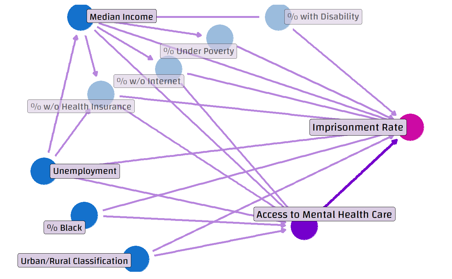
In order to isolate the relationship between access to mental health care and imprisonment rate, I examined the potential variables that may confound the results. Data for many characteristics of census tracts are available, including the percent of residents with a disability, the percent under the poverty level, the percent without internet access at home, and the percent without any health insurance. However, all of these variables are so closely related to median income and unemployment rates that their impact is accounted for when I control for median income, unemployment rate, the percent of Black residents, and the tract’s urban/rural classification. The diagram in Figure 1 displays the directional logic of the model.
I use a multilevel Bayesian regression model to examine both the influence of the control variables and the variation within and between each county in Maryland. The Bayesian method differs from the common frequentist methods because these models will draw 10,000 iterations of the model (the first 5,000 draws are discarded as warm up), and I will assess the probability of direction for the coefficients in each model. Instead of statistical “significance,” I will discuss the results in terms of probability of direction based on the distribution of coefficients. I have included complete formal specifications of all models, likelihoods, and priors in the appendix.
Multilevel Model
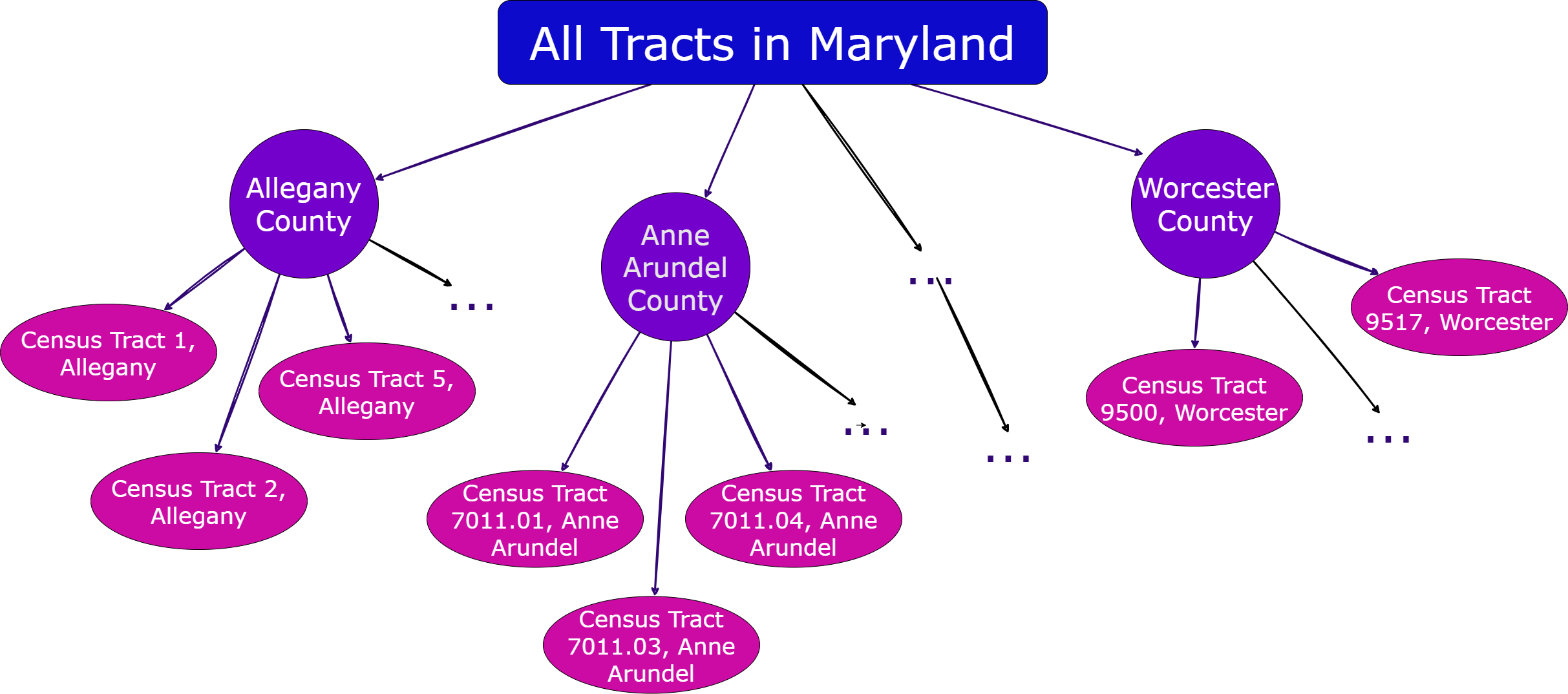
I use a multilevel modeling approach to capture the variation both between and within each county. In other words, I want the model to consider the distribution of relationships within each county to inform the prediction for a specific tract; I also want to consider the variability between counties. In a way, this county-level random effects modeling approach considers the surrounding area, which variables are related to imprisonment rates, and how similar or different those relationships are within and between counties. Figure 2 provides a simplified diagram of the hierarchical levels in the model.
\[ \begin{aligned} \text{Layer 1:} & Y_{ij} | \mu_j, \sigma_y \sim \text{model of how imprisonment varies WITHIN counties } j \\ \text{Layer 2:} & \mu_j | \mu, \sigma_\mu \sim \text{model of how the typical imprisonment} \mu_j \text{varies BETWEEN counties.} \\ \text{Layer 3:} & \mu, \sigma_y, \sigma_\mu \sim \text{prior models for shared global parameters} \\ \\ i = & \text{Tract} \\ j = & \text{County} \\ \end{aligned} \]
Established indicators
(demographics and socioeconomic factors)
The first equation includes only the demographic and socioeconomic factors as the established indicators for high imprisonment rates. This model provides us with a baseline of the relationship between these established indicators and imprisonment rates in Maryland.
\[ \begin{aligned} Y_{ij} | \beta_{0j}, \beta_1, \beta_2, \beta_3, \beta_4, \sigma_y \sim N(\mu_{ij}, \sigma_y^2) \;\; \text{ with } \;\; \mu_{ij} =& \beta_{0j} + \\ &\beta_1\text{Percent Black}_{ij} + \\ &\beta_2\text{Median Income}_{ij} + \\ &\beta_3\text{Unemployment Rate}_{ij} + \\ &\beta_4\text{Urban}_{ij} \\ \\ \beta_{0j} | \beta_0, \sigma_0 \stackrel{ind}{\sim} & N(\beta_0, \sigma_0^2) \\ \beta_{0c} \sim & N(100, 10^2) \\ \beta_1 \sim & N(100, 60) \\ \beta_2 \sim & N(-50, 15) \\ \beta_3 \sim & N(100, 25) \\ \beta_4 \sim & N(100, 25) \\ \sigma \sim & \text{Exp}(l) \\ \sigma_y \sim & \text{Exp}(0.072) \\ \sigma_0 \sim & \text{Exp}(1) \\ \end{aligned} \]
Proximity to mental health facilities
Since each tract has three variables regarding distance to facilities and two measures of distance (miles and minutes), a total of six models for each equation were evaluated—distance in time and miles to any mental health facility, distance in time and miles to an inpatient mental health facility, and distance in time and miles to an inpatient mental health facility with crisis intervention. The first of these equations examines the relationship between distance (miles and minutes) and imprisonment without any controls.
The second equation is the same but controls for urban/rural classification of the tract. (Since each housing unit is classified as urban or rural and the data from the US Census provides the number of housing units in each trach and the counts for urban and rural classification, tracts were coded for this analysis as urban only when they contained no rural housing units. The high bar for urban classification comes from the higher number of urban tracts and the average size of census tracts is a relatively small unit of analysis; to even the numbers out, only 100% urban tracts are coded as urban, resulting in 1005 tracts coded as urban and 420 tracts coded rural for this analysis). The third equation combines all of the established indicators from the baseline model and distance to each type of facility.
\[ \begin{aligned} Y_{ij} | \beta_{0j}, \beta_5, \sigma_y \sim N(\mu_{ij}, \sigma_y^2) \;\; \text{ with } \;\; \mu_{ij} =& \beta_{0j} + \\ &\beta_5\text{Distance to Facility}_{ij}\\ \\ Y_{ij} | \beta_{0j}, \beta_4, \beta_5, \sigma_y \sim N(\mu_{ij}, \sigma_y^2) \;\; \text{ with } \;\; \mu_{ij} =& \beta_{0j} + \\ &\beta_4\text{Urban}_{ij} + \\ &\beta_5\text{Distance to Facility}_{ij} \\ \\ Y_{ij} | \beta_{0j}, \beta_1, \beta_2, \beta_3, \beta_4, \beta_5, \sigma_y \sim N(\mu_{ij}, \sigma_y^2) \;\; \text{ with } \;\; \mu_{ij} =& \beta_{0j} + \\ &\beta_{1-4}\text{Established indicators}_{ij}\\ &\beta_5\text{Distance to Facility}_{ij}\\ \end{aligned} \]
Analysis
Summary and Overview of the Data
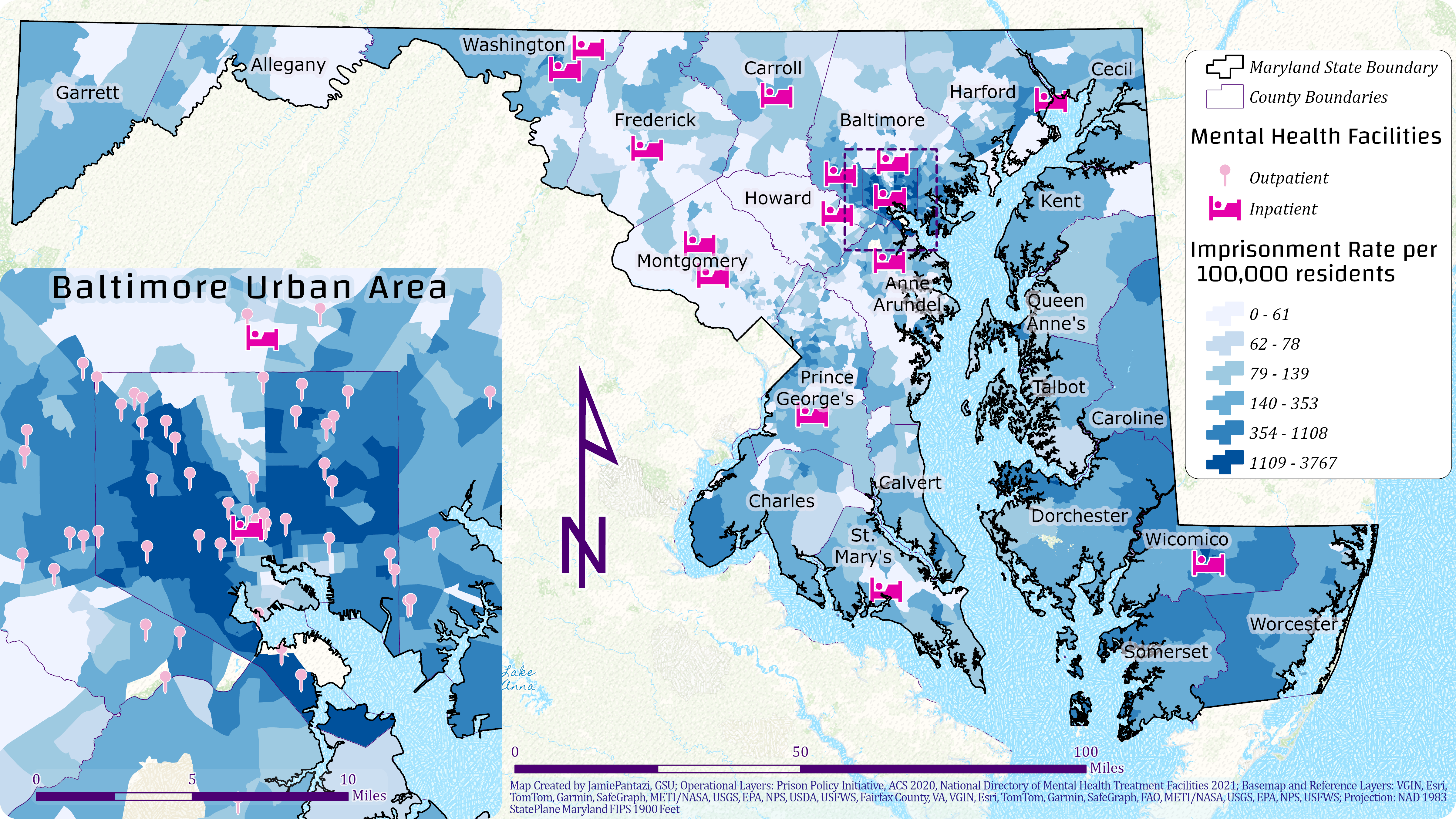
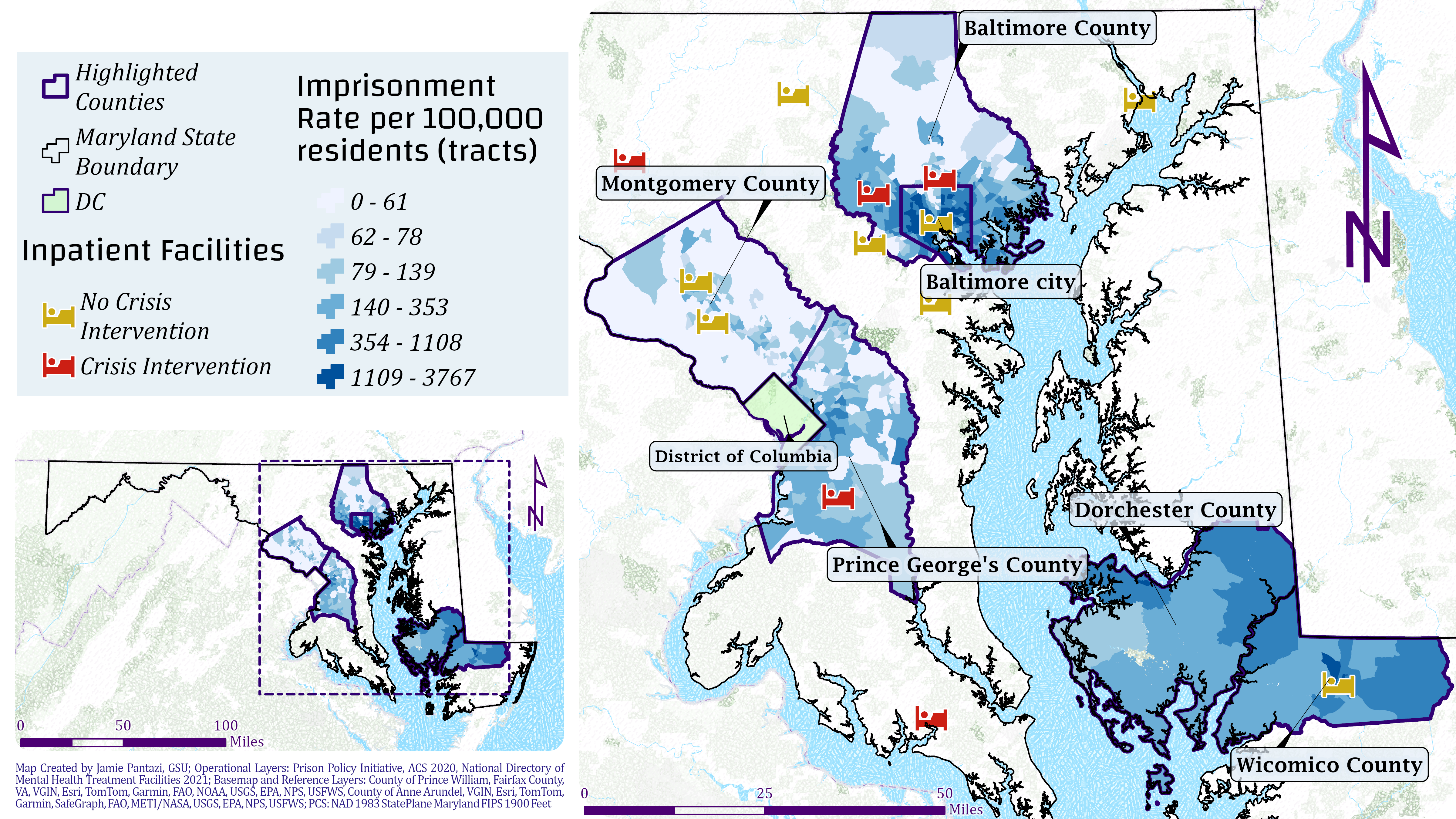
Before interpreting the results from these models (visualizing the primary variables, imprisonment rate and inpatient mental health facilities) on a map provides some preliminary context for greater research questions. The map of imprisonment rates in Maryland, shown in Figure 3, highlights the concentration of high imprisonment in the Baltimore urban area. Since Baltimore is the largest urban area entirely in Maryland, it is not unexpected to see higher rates of imprisonment in the city and surrounding areas. However, the suburbs of Washington, D.C. are also partially in Maryland with comparable population density, but the imprisonment rate for those areas are much lower than the Baltimore suburbs. Though rural areas outside of the two major metropolitan areas seem to have lower rates of imprisonment overall, the southeast peninsula and northwest panhandle seem to have surprisingly higher rates. From this map, it seems that these areas are further from inpatient facilities, and the few in those areas may not have sufficient capacity for the large areas they serve.
| Tract Characteristics | |||||
| Mean | Median | Std Dev | Min | Max | |
|---|---|---|---|---|---|
| Imprisonment Rate per 100,000 | 314 | 139 | 497 | 0 | 3,767 |
| Total Population | 4,104 | 3,911 | 1,603 | 776 | 11,509 |
| Median Income | $107,055 | $101,406 | $44,815 | $14,464 | $250,001 |
| % Black | 31.0% | 18.5% | 30.2% | 0.0% | 99.7% |
| Unemployment Rate | 5.5% | 4.5% | 3.9% | 0.0% | 31.2% |
| % Rural | 14.9% | 0.0% | 32.1% | 0.0% | 100% |
Table 3 summarizes some key variables regarding census tract characteristics in the new dataset. The median income across all tracts in Maryland was $101,406, compared to a national median income of $62,529. The average percentage of Black residents for each tract was 31.0%, compared to only 11.2% nationwide. As a mid-atlantic state, tracts in Maryland have a lower percentage of rural housing than the national average by about half.
| Distance to Nearest Facility | |||||
| Mean | Median | Std Dev | Min | Max | |
|---|---|---|---|---|---|
| Driving Miles to Mental Health Facility | 4.3 | 2.7 | 5.0 | 0.1 | 51.8 |
| Travel Time to Mental Health Facility | 9 min | 8 min | 7 min | 1 min | 74 min |
| Driving Miles to Inpatient Facility | 12.0 | 8.7 | 13.8 | 0.2 | 119.9 |
| Travel Time to Inpatient Facility | 22 min | 19 min | 15 min | 1 min | 139 min |
| Driving Miles to Inpatient Facility with Crisis Intervention | 22.3 | 16.6 | 24.7 | 0.4 | 152.4 |
| Travel Time to Inpatient Facility with Crisis Intervention | 36 min | 30 min | 29 min | 2 min | 184 min |
The key additional variables calculated and added to the dataset are the distances from each census tract to the closest mental health facility with various characteristics. By identifying various measures of access by distance for each tract, this new dataset may offer unique insights about which communities are most in need of investment in mental health well-being and crisis response. As seen in Table 4, the average distance throughout the state is not extreme; the average travel time to any facility is less than ten minutes, and under thirty minutes to inpatient facilities with crisis intervention. However, some tracts are up to 74 minutes away from any mental health facility, 139 minutes from inpatient facilities, and up to almost three hours from an inpatient facility with crisis intervention. For communities in these areas, the only available response to crisis may be the police, which can lead to more harm to an individual in need of mental health services and those around them.
| Facility Characteristics | ||||
| All | Count | Inpatient | Count | |
|---|---|---|---|---|
| Inpatient Services | 8.6% | 20 | 100% | 20 |
| Outpatient Services | 86.7% | 202 | 60.0% | 12 |
| Partial Hospitalization Services | 17.2% | 40 | 90.0% | 18 |
| Residential Services | 13.3% | 31 | 5.0% | 1 |
| Telehealth Services | 65.7% | 153 | 35.0% | 7 |
| Serves Adults | 88.0% | 205 | 90.0% | 18 |
| Crisis Intervention | 30.0% | 70 | 50.0% | 10 |
| Walk-ins Accepted | 18.9% | 44 | 65.0% | 13 |
| Federally Qualified Health Center | 11.2% | 26 | 0.0% | 0 |
| Accepts Medicaid | 93.6% | 218 | 100% | 20 |
| Accepts Medicare | 69.1% | 161 | 100% | 20 |
| Payment Assistance | 17.6% | 41 | 5.0% | 1 |
| Sliding Scale | 35.6% | 83 | 5.0% | 1 |
Of all facilities in Maryland, only 8.6%, or 20 facilities, offer inpatient care. Table 5 shows the frequency and percentages of various services and payment options. Most of these characteristics will not be covered in-depth in this report; the primary focus will be inpatient facilities with crisis intervention. The larger issue of inadequate mental health outpatient care and cost-prohibitive preventative care is another dimension of the story about the interactions of mental health and imprisonment that could also be explored with these data given the new variables available.
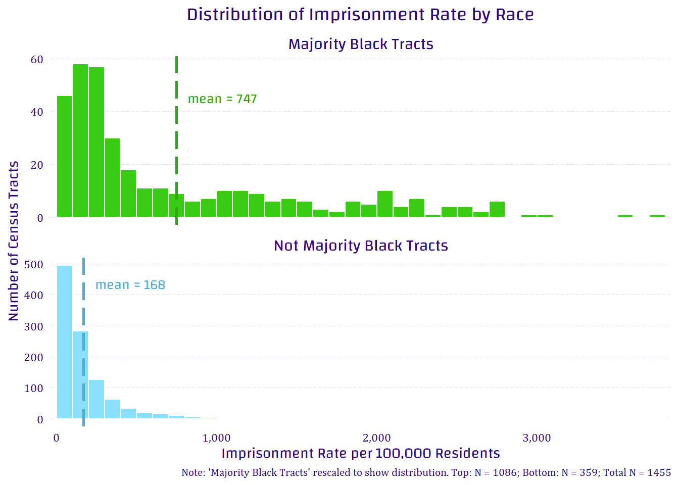
An initial overall look at the distribution of the tracts and imprisonment rate shows that a clear and obvious characteristic related to higher rates is race. Figure 4 clearly shows that census tracts that have a majority Black population have, on average, much higher rates of imprisonment. Tracts with less than a majority Black population had an average imprisonment rate of 168, and majority Black tracts had an average of 747, or 580 higher than their counterparts. While majority Black tracts had over 100 tracts with an imprisonment rate above 1,000 per 100,000 people, tracts without a majority Black population had only eight above 1,000 per 100,000 people (see Table 6).
| Outliers | |||
| FIPS Code | Tract | Imprisonment Rate | % Black |
|---|---|---|---|
| 24043000400 | Census Tract 4, Washington County, Maryland | 1,743 | 40.5% |
| 24510250401 | Census Tract 2504.01, Baltimore city, Maryland | 1,263 | 27.2% |
| 24510250303 | Census Tract 2503.03, Baltimore city, Maryland | 1,168 | 23.1% |
| 24510260404 | Census Tract 2604.04, Baltimore city, Maryland | 1,139 | 11.4% |
| 24510250500 | Census Tract 2505, Baltimore city, Maryland | 1,115 | 39.2% |
| 24510060300 | Census Tract 603, Baltimore city, Maryland | 1,096 | 36.1% |
| 24510060200 | Census Tract 602, Baltimore city, Maryland | 1,030 | 47.5% |
| 24510030200 | Census Tract 302, Baltimore city, Maryland | 1,009 | 26.5% |
Bayesian Regression
Established indicators
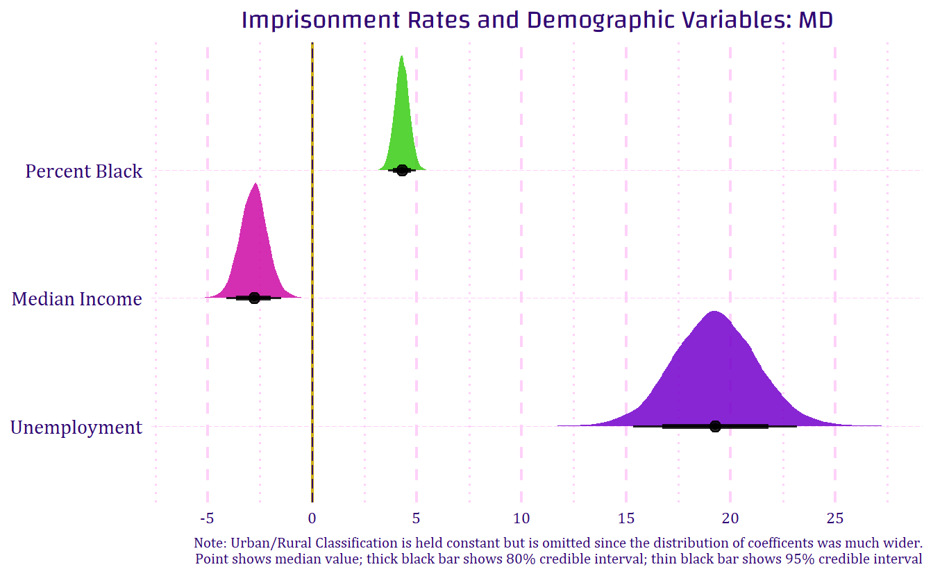
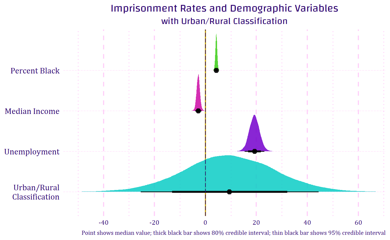
The first model examines the relationship between the percent of Black residents, median income, unemployment rate, and urban/rural classification with imprisonment rate per 100,000 residents by census tract. Using the hierarchical model explained earlier, I am taking into account the variation of imprisonment rate within and between counties to return a more precise estimate. The results indicate a positive correlation between the percent of Black residents and imprisonment rates (with a median coefficient of 4.3 and an entirely positive distribution), a negative correlation for median income (with a median coefficient of -2.8 and an entirely negative distribution), and a very positive correlation for unemployment rate (with a median coefficient of 19.2 and an entirely positive distribution); the urban rural classification of the census tract did not have a meaningful correlation with imprisonment rate when controlling for these other variables (the median coefficient was 9.3); even the 80% credible interval was spread well below and above zero (-12.4 and 32.7). The probability of a positive relationship between urban classification and imprisonment is only 70.6%.
Figure 5 shows the distribution of the coefficients for each variable throughout the iterations of the model. It is not unsurprising that areas with higher concentrations of Black and poor residents have higher imprisonment rates. Additionally, since unemployment rates impact lower income communities more, some of the statistical correlation may be obscured by the income variable. It is important to note that, though most crime is associated with urban areas, and imprisonment should be associated with crime, no significant difference was found between imprisonment rates in rural tracts and urban tracts when controlling for race and income (see Figure 6).
Taking a closer look into the variation by location in the state, or county, I have selected three pairs of neighboring counties to examine—Baltimore city and Baltimore county, Montgomery and Prince George’s counties (DC suburbs), and Dorchester and Wicomico counties (rural peninsula). With a reputation for high rates of violent crime, Baltimore city has been the topic of crime and policing in many discussions on the issue, but Baltimore county, which surrounds Baltimore city on all sides without a water border, is a very different place in terms of demographics and imprisonment.
The two DC suburbs, Montgomery and Prince George’s counties, actually have a greater disparity in the percent of Black residents than Baltimore city and Baltimore county, and an almost identical income disparity. However, Baltimore city has almost twice the unemployment and almost four and half times the imprisonment rate as Baltimore county; the imprisonment and unemployment disparity between the suburban DC counties is not as severe. The two rural peninsula counties were chosen because they had imprisonment rates higher than other rural areas. When comparing these rural counties with the other pairs, they stand out as having a lower percent of Black residents than the other counties (save Montgomery county). However, these rural counties also have a lower median income than all the other selected counties (including Baltimore city), and a higher unemployment rate than all but Baltimore city (see Table 7).
| Selected Counties | ||||
| County | Imprisonment Rate | Percent Black | Median Income | Unemployment Rate |
|---|---|---|---|---|
| Baltimore Metro Area | ||||
| Baltimore City | 1,167 | 63.0% | $73,963 | 8.7% |
| Baltimore County | 260 | 27.3% | $101,468 | 4.9% |
| DC Suburbs | ||||
| Montgomery County | 63 | 18.0% | $140,741 | 4.6% |
| Prince George's County | 174 | 63.3% | $101,367 | 6.5% |
| Rural Peninsula | ||||
| Dorchester County | 511 | 23.8% | $67,102 | 7.3% |
| Wicomico County | 688 | 28.8% | $72,223 | 7.7% |
Figure 7 shows the linear relationship between median income and imprisonment rate in several selected counties. The most noticeable correlations between income and imprisonment can be seen in the plots for Baltimore city and the two rural peninsula counties, Dorchester and Wicomico. The slopes for the suburban counties around DC are almost entirely flat, and there is only a slight downward slope for Baltimore county. Figure 8 shows these counties on the map to provide spatial context for these relationships.
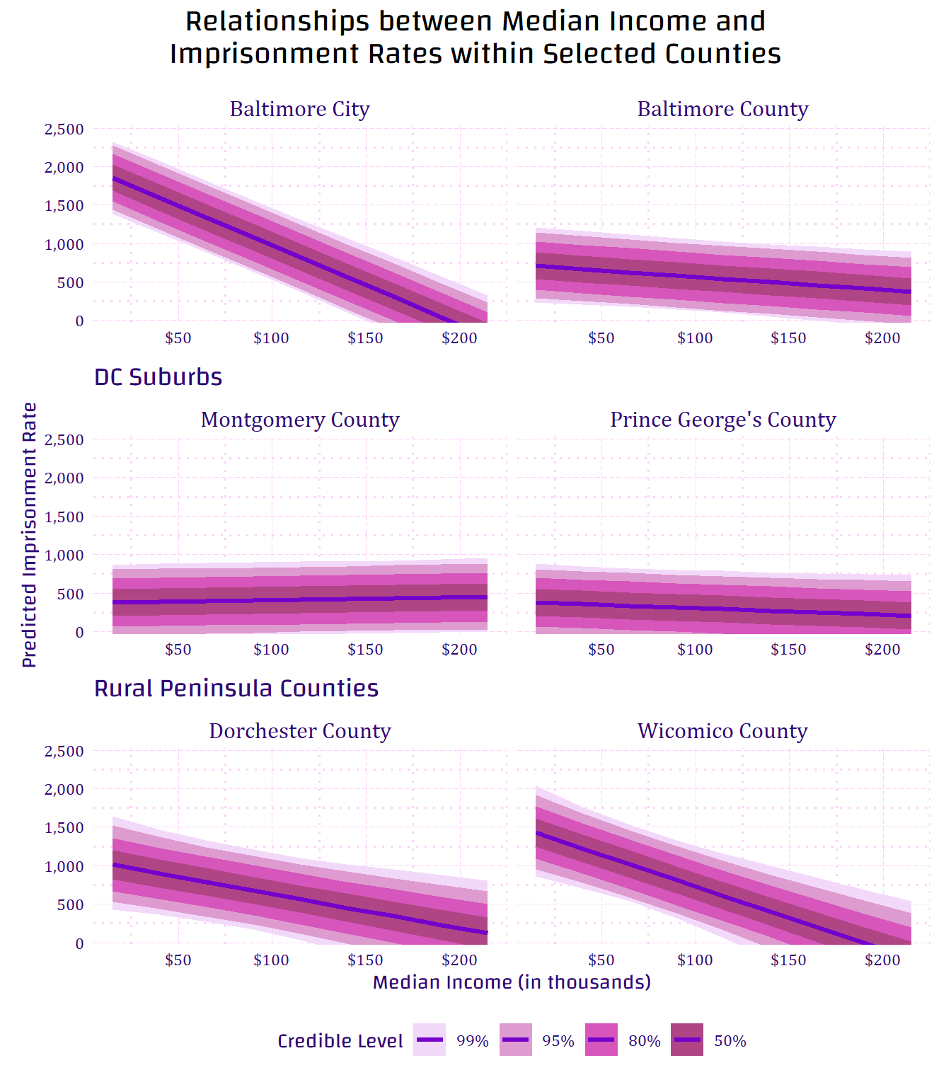
It is interesting to note that Prince George’s county has an almost identical share of Black residents as Baltimore city but only 15% of the imprisonment rate. The median income for Prince George’s was also much higher than Baltimore city ($101,367 versus $73,963), and this calls into question whether income, once it reaches a minimum median, does it cancel the impact of the racial makeup of an area? This question is outside the scope of this research, but comparing these counties side by side may indicate that income, or the median income of an area, once it reaches a certain point, may reduce imprisonment rates.
Distance
Because urban tracts are overrepresented and more likely to be spatially close to a facility, the relationship is not clear. However, this does not account for capacity at urban facilities. Even assuming the one facility in Baltimore may have a higher capacity than average, it is unlikely the one inpatient facility (without crisis intervention) within Baltimore City is equipped to adequately provide care to the city’s nearly half a million people. The map from Figure 3 highlights that Baltimore has the highest concentration of high imprisonment rates in Maryland, but only one facility offering inpatient care for a large and densely populated area.
Since each tract has three variables regarding distance to facilities, three models for each equation were evaluated— (1) distance to any mental health facility, (2) distance to an inpatient mental health facility, and (3) distance to an inpatient mental health facility with crisis intervention. Figure 9 shows the distribution of coefficients for distance to facilities only, as it correlates with imprisonment rates. In the case of each type of facility, the correlation is either negative or unclear, but this is expected without any controls. Because the facilities, especially mental health facilities generally, act as a proxy for population density, and densely populated areas have a higher police presence and thus higher imprisonment rates, distance alone is not enough to determine any meaningful relationship between access to mental health care and imprisonment.
According to this model, each driving mile to a mental health facility from the center of a census tract is associated with a median 17.2 decrease in imprisonment rate per 100,000 residents in that tract, and I can be 99.9% certain that the relationship is negative. Each mile to an inpatient facility is associated with a median 7.5 decrease, and I can be 91.6% certain that the relationship is negative; each mile to an inpatient facility with crisis intervention services is associated with a median 0.2 decrease, and I am only 55.0% certain that the relationship is negative (see Figure 9).
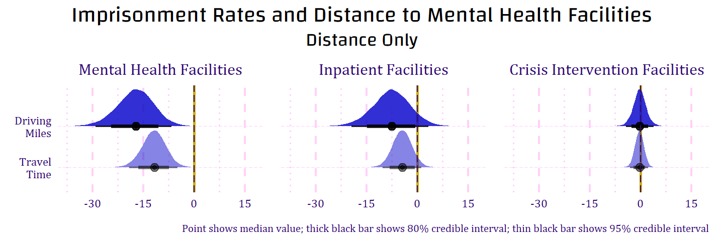
Each driving mile to a mental health facility from the center of a census tract is associated with a median 14.3 decrease in imprisonment rate per 100,000 residents in that tract, and I can be 99.6% certain that the relationship is negative. Each mile to an inpatient facility is associated with a median 6.6 decrease, and I can be 89.3% certain that the relationship is negative; each mile to an inpatient facility with crisis intervention services is associated with a median 0.9 increase, but I can be only 70.3% certain that the relationship is positive.
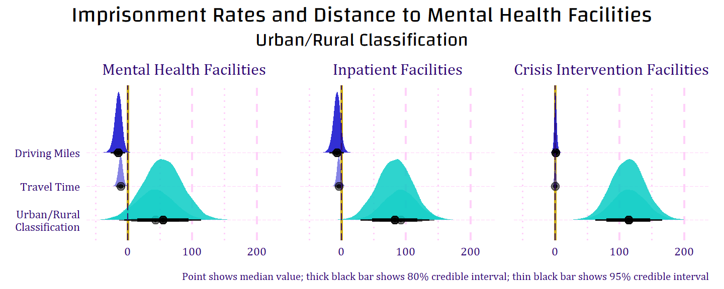
Without the demographic controls (percent Black, median income, and unemployment rate), an urban classification corresponds to a median coefficient of 54 when controlling for distance to any mental health facility, and I can be 96.2% that the relationship is positive. When I control for inpatient and crisis intervention facilities, the relationship between urban classification is even more certain— a median coefficient of 83 when controlling for distance to an inpatient facility, 114 for distance to a facility with crisis intervention, and I can be 100.0% certain that the relationships are positive (see Figure 10).
When I add the demographic variables back into the model with distance, each driving mile to a mental health facility from the center of a census tract is associated with a median 4.1 decrease in imprisonment rate per 100,000 residents in that tract, and I can be 88.6% certain that the relationship is negative. Each mile to an inpatient facility is associated with a median 4.8 decrease, and I can be 83.4% certain that the relationship is negative; each mile to an inpatient facility with crisis intervention services is associated with a median 4.5 increase, and I can be 96.2% certain that the relationship is positive (see Figure 11).
The results with all controls do alter the degree of correlation with the control variables. These models indicate a higher positive correlation between the percent of Black residents and imprisonment rates with a median coefficient of 6.1 for distance to any mental health facility, 6.7 for inpatient, and 7.1 for facilities with crisis intervention. The negative correlation between median income and imprisonment rate does shrink a bit, with a median coefficient of -1.7 for distance to any facility, -1.5 for inpatient, and -1.3 for facilities with crisis intervention, but I can still be 100.0% certain the relationship is negative for all three models. The positive correlation for unemployment rate (already the most correlated variable without controlling for distance) becomes even more apparent in these models, with median coefficients of 27.8, 25.6, and 26.7, I can be 100.0% certain the relationship is positive for all three models.
The urban classification of the census tract still did not have a meaningful correlation with imprisonment rate when controlling for these other variables (the median coefficients were -23.5 for any facilities, -19.8 for inpatient, and -6.6 for crisis intervention). The distribution for urban/rural classification has been left off of Figure 11 since it is much wider than the others and does not contribute meaningful results. The probability of a positive relationship between urban classification and imprisonment is only 15.4% for any facilities, 17.9% for inpatient, and 38.1% for crisis intervention.
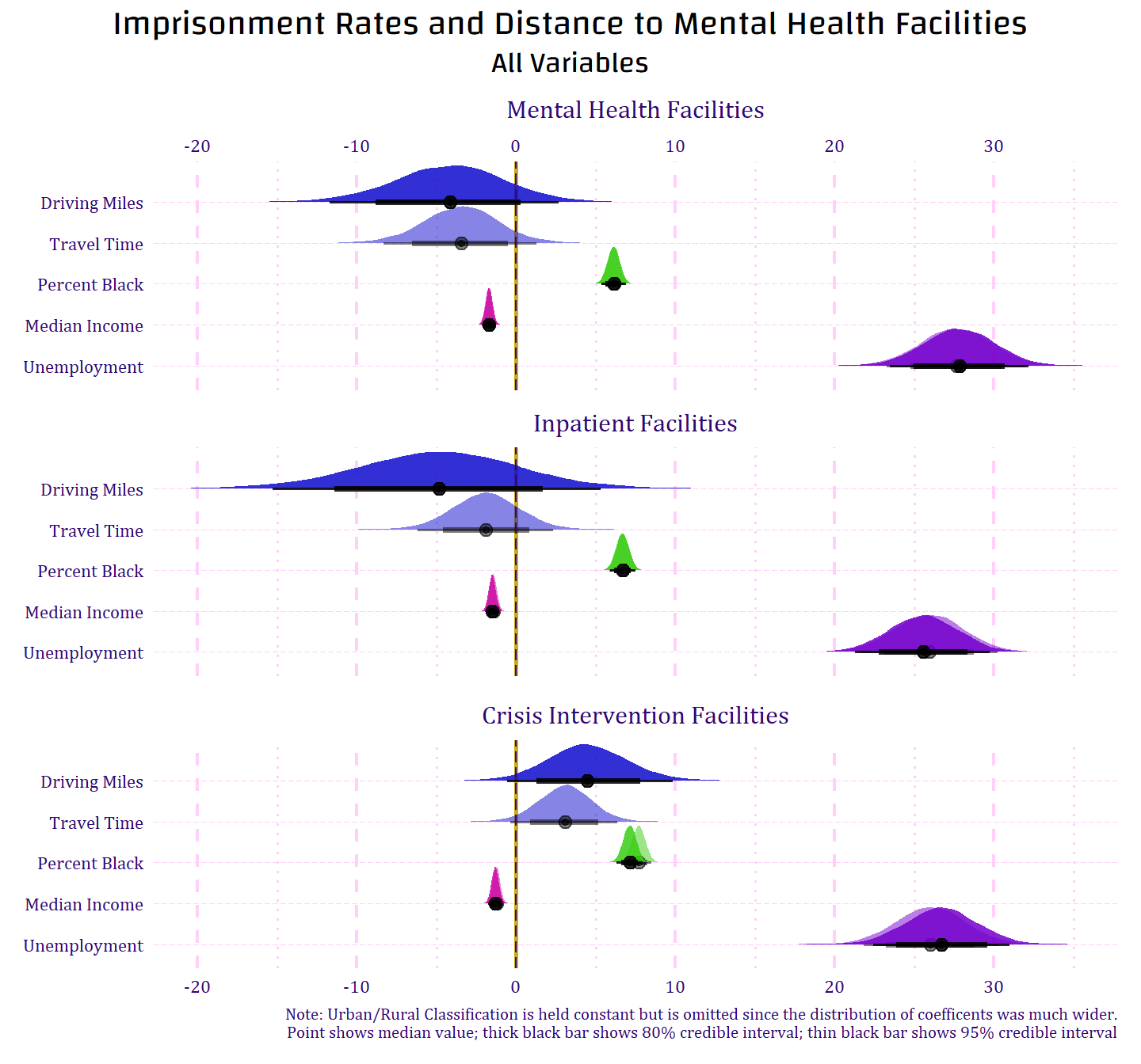
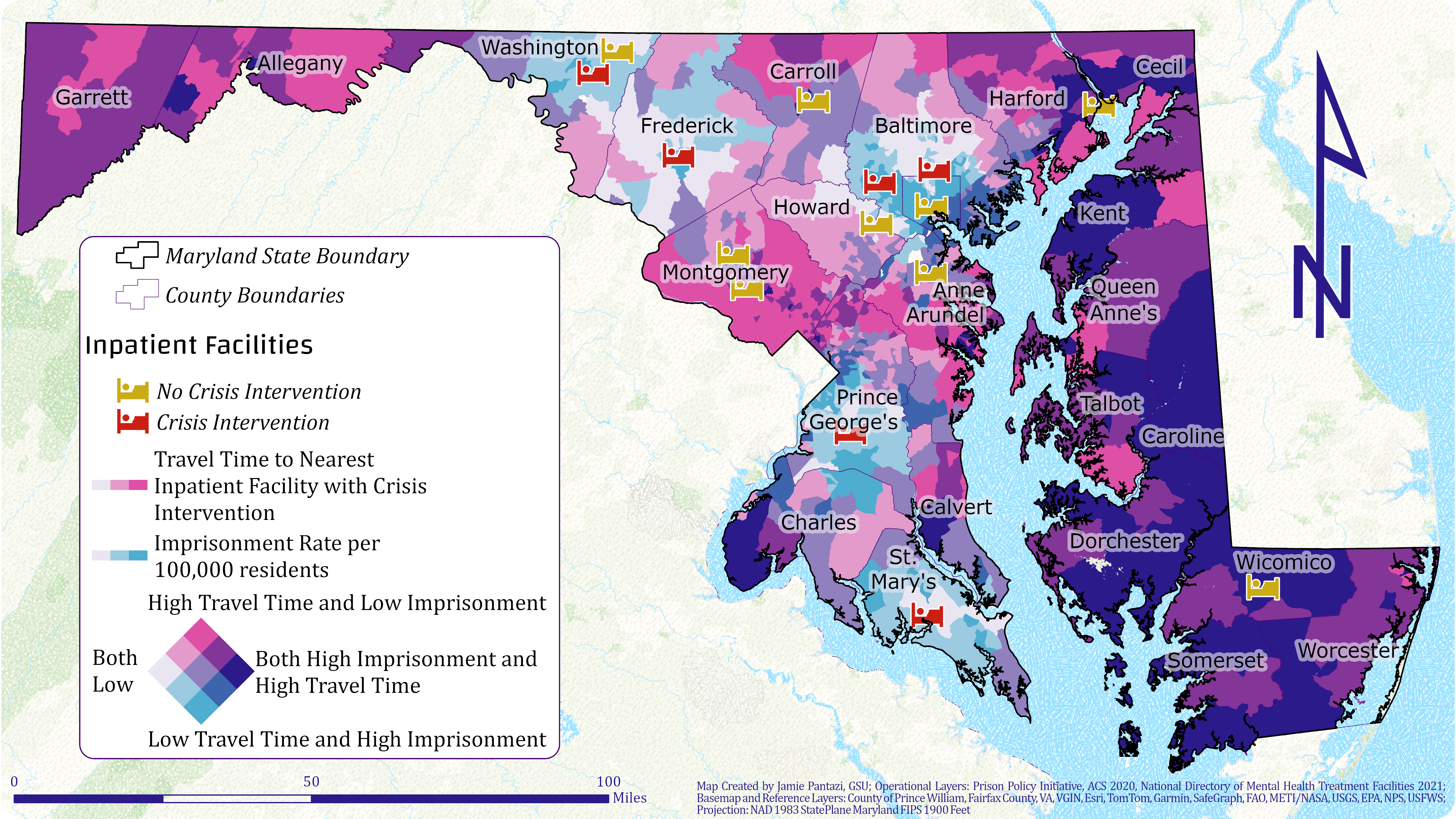
Figure 12 displays the spatial representation of distance to mental health facilities with crisis intervention and imprisonment rates. Each variable is represented by a different color and as they increase the color is darker, and when they overlap the color darkens and changes. This map helps to orient the spatial relationship and identify areas that may benefit from more available mental health care, especially crisis intervention.
Discussion
Although the results of this analysis are not overwhelmingly conclusive regarding the distance to facilities, this research does confirm that the established indicators about race, income, and unemployment have precise and noteworthy associations with imprisonment rates. It may be important to note that, though distance itself may not have a meaningful correlation with imprisonment, when I control for distance, the unemployment rate becomes more influential. Unemployment in the first model (without distance) had a median coefficient of 19.2, and that increased to 27.8 in the any facilities model, 25.6 in the inpatient model, and 26.7 in the crisis intervention model; that is an average increase of 7.5 imprisoned people per 100,000.
Additionally, the coefficients for my robustness check using travel time to the nearest facility in minutes did not make any meaningful difference to any other variables, and the coefficients for travel time were actually distributed more narrowly, suggesting that travel time may be a more accurate measure that distance in miles.Additionally, the coefficients for my robustness check using travel time to the nearest facility in minutes did not make any meaningful difference to any other variables, and the coefficients for travel time were actually distributed more narrowly, suggesting that travel time may be a more accurate measure that distance in miles.
Without data about the capacity of these facilities to compare to the population densities in their area, distance alone is just not a sufficient measure of access to care. Other than the further contribution about demographic and socio-economic status influencing who is imprisoned (a well-tread area of research), this analysis mostly leaves us with more questions. While capacity is certainly an important attribute to consider, there are many other barriers to accessing mental health care—lack of insurance, dependents that rely on you, financial demands that are prioritized over the time and energy investment of finding appropriate care, the list goes on.
Limitations
The primary limitation in this analysis is the lack of data about facility capacity, especially for inpatient facilities. Many inpatient facilities have very few beds, and the few with higher capacity are generally poorly funded and staffed, rendering them unable to provide meaningful treatment to patients. While the issue of unknown capacity limits the significance of this analysis, it also speaks to a larger issue around transparency in the mental health industry. As a consumer of mental health services, especially inpatient services, very little agency or informed choice (or consent) exists when seeking out these services. In a general medical situation, one has access and information about available treatments and the details of those treatments before they seek them out. However, when examining the publicly available information from mental health providers, especially inpatient facilities, little specifics exist about the nature of available treatments at a given facility. Websites for these facilities generally offer vague bullet points about the kinds of mental health diagnoses they treat and maybe a list of general therapeutic practices.
On the website for one facility, the only information regarding inpatient care provided was that it is “a secure nursing unit that provides short term acute care, overnight medical treatment and therapy to patients who need life-saving care for their behavioral health condition” (UM Baltimore Washington Medical Center, n.d.). Another facility’s website reads, “Our safe spaces are created to promote comfort, healing, and privacy for our patients. We provide personalized, collaborative care to patients with serious and recurring mental health disorders that may include:” and goes on to list several common mental health disorders (University of Maryland School of Medicine, n.d.). In the best cases, facilities may list a variety of therapeutic methods such as “Cognitive Behavioral Therapy,” “Dialectical Behavioral Therapy,” or “Mindfulness-Based Therapies,” but the variation in these methods is immense, so there is no way to really know what those therapies will look like in practice (MedStar Health, n.d.). Speaking from personal experience with several inpatient facilities, both for my own care and the care of a loved one, I have seen how deceptive and evasive the intake process can be (even as far as being directly lied to in order to gain my consent). Asking questions about the care or requesting any kind of agency over the kind of care you are seeking is nearly impossible; if you are deemed a threat to yourself or others by whichever underpaid intake staff has a shift when you arrive, you can be held without consent, and there is no recourse.
I took myself to a facility on one occasion when I was suffering from severe suicidal ideations, no plan just thoughts, and it had worsened over the weekend. I was concerned about being home alone on Monday when my partner would be at work. I found a facility in my area with an intensive outpatient program; this would provide me a safe place to be during the day when I would otherwise be alone. I had been depressed for a while, and probably not taking the best care of myself, so I did not look my best when I arrived at the facility on a Sunday evening. Upon entering the building, they took mine and my partner’s phones and personal items and locked them in a closet. After a very judgmental woman completed an intake questionnaire with me, without allowing my partner to be present, she left me alone and scared. I had told her that I wanted to do the partial hospitalization program because I had completed a program like that in the past, and it was helpful. When she came back she told me that I was recommended for impatient treatment. I told her I did not want inpatient treatment, and at that time she told me that I did not have a choice, and if I refused, the police would get involved and they would force me to stay. When I asked why I had to accept inpatient treatment, she would not give me any details other than that my hair was unkempt. After two days in jail-like conditions, I was finally seen by a doctor who concluded I did not need inpatient care, and recommended that I participate in the partial hospitalization program.
Transparency
The lack of transparency and informed consent surrounding mental health, especially inpatient care, is disturbing for several reasons: the legacy of deinstitutionalization has not been adequately addressed, the utilization of mental health care is rising, and, in part because of deinstitutionalization, funding to mental health care is slim to say the least.
Deinstitutionalization refers to the era in the 1980s when the Reagan Administration gutted funding for large mental institutions and replaced them with block grants to the states which resulted in many facility closures, leaving their patients to fend for themselves (Perry, 2016). Schutt aptly describes the implications and impacts concluding that “Deinstitutionalization in the absence of socially supportive programs has been associated with increased rates of homelessness and incarceration among those most chronically ill” (Schutt, 2016).
The Mental Health Parity and Addiction Equity Act of 2008 mandated that behavioral health care must be covered by health insurance equal to general medical care, which gave access to mental health care to many people for the first time (Internal Revenue Service, Department of the Treasury et al., 2010). Since 2008 the rate of people in the US utilizing mental health care has steadily risen since the Mental Health Parity Act went into effect in 2010 (Wang et al., 2023).
Prior to last year’s historical reform to eliminate cash bail in Illinois, The Atlantic called out the outrageous rates of mental health needs in the Cook County Jail (Ford, 2015; Illinois Safety, Accountability, Fairness and Equity-Today (SAFE-T) Act, 2021). A study in 2010 found that there were “now more than three times more seriously mentally ill persons in jails and prisons than in hospitals” (Torrey et al., 2010). Despite the success of the Mental Health Parity Act, federal and state governments have failed to provide adequate funding for mental health providers and institutions (Kennedy-Hendricks et al., 2018; Mahomed, 2020). The average salary for mental health care providers, in both the private and public sector, is only marginally higher than correctional officers according to GlassDoor.com ($46K - $71K/year for mental health care providers versus $39K - $56K/year for correctional officers) (Salary, n.d.-a, n.d.-b).
Transparency is increasingly important as access and availability of mental health care is being pushed as an alternative to incarceration because we want to know that individuals are actually getting the care they need and not allowing mental health facilities to turn into a new brand of confinement for society’s “undesirables” (as was often true of the original asylums for the mentally ill in the United States) (Whitaker, 2019).
Further Research
The new datasets and insights from this analysis open up many more research questions to explore. Some have already been mentioned but would require cooperation with the facilities providing care. The question of capacity is a critical one to investigate, but perhaps a more important issue (and more difficult) might be the question of quality of the care received at the limited place available. While this research hopes to provide insights into alternatives to carceral punishment, it should not be misunderstood that the goal is not to empty the prisons only to detain the same people in mental health facilities. Mental health care can be helpful to prevent harm and to heal from harm, but the care must be adequate, accessible, and appropriate for the individuals seeking support. Further research should consider the quality of care, even if it is not the main focus.
One interesting insight discussed earlier may warrant further investigation. We know race is highly related to imprisonment, but by examining these trends on county and census tract levels, it seems there may be a threshold of median income for an area that cancels out the impact of race. The county-level random effects in the model without proximity showed an almost flat slope for the suburban DC counties. Prince George’s county has a higher percentage of Black residents than Baltimore city (and a comparable income disparity with its neighboring majority white county), but a much lower imprisonment rate. Is this because Prince George’s county has an inpatient facility with crisis intervention (and probably a less dense population), or is it the higher median income that is primarily driving down imprisonment rates (or interactions with police in the first place)? Perhaps there is a threshold of median income where race is no longer a reliable indicator of imprisonment. If Black people live in an area with primarily other Black people, how much money do they need to make on average to keep the police out of their neighborhoods?
Another important question that warrants further analysis with these unique dataset concerns issues facing individuals after they are released from prison. Presumably, they will return to the communities from which they were removed, and they are likely to experience increased barriers to mental health care. Their criminal record alone is likely to diminish employment opportunities (often in areas where unemployment rates are well about the average). Even when gainful employment and health insurance are possible, the stigma and traumatic consequences of seeking mental health care within prison culture can prevent many from seeking care even when it is available long after they are released. Using this spatial data to identify places most in need of re-entry support will be an important component of fighting the cycle of harm caused by the prison industrial complex. Similarly, these same areas can be targeted for increased mental health (and material) support for the families left behind in these communities when a loved one is sent to a cage sometimes hundreds of miles away with no means to provide financial or emotional support.
Datasets:
In addition to the insights discussed in this paper, this research has also produced two useful datasets, as well as the process for creating these datasets for different states (see appendix for R code and ArcGIS Pro logs):
- Maryland facilities list with their characteristics according to the SAMHSA’s National Directory of Mental Health Treatment Facilities 2021
- Maryland tracts with nearest facilities (mental health, inpatient, and inpatient with crisis intervention) and the other characteristics for each of the nearest facilities in each category
Conclusion
Though the results of this research are not overwhelmingly novel or conclusive in answering our research question, the difficulty obtaining the necessary information about capacity (or anything else) has illuminated a greater issue of transparency around mental health care. Future researchers should continue to press these institutions to increase transparency to enable researchers and the greater public to analyze and assess their work and impact.
Warning
I would like to conclude with a disclaimer to future researchers and policymakers who will help shape the future of mental health care. While I am advocating for mental health care and treatment as an alternative to imprisonment and detention to combat violence and other harms to community members, the quality of care is equally important, albeit much more complex and difficult to measure. In no uncertain terms, I want to warn against the threat of profit-driven agendas that would be happy to rehouse those they deem “criminals” in mental health hospitals instead of prisons. As advocates of alternatives to detention, we must not be appeased by these attempts to placate our demands with a mere vocabulary adjustment; “a rose by another name” is not progress.
Appendix
Established indicators
\[ \begin{aligned} Y_{ij} | \beta_{0j}, \beta_1, \beta_2, \beta_3, \beta_4, \sigma_y \sim N(\mu_{ij}, \sigma_y^2) \;\; \text{ with } \;\; \mu_{ij} =& \beta_{0j} + \\ &\beta_1\text{Percent Black}_{ij} + \\ &\beta_2\text{Median Income}_{ij} + \\ &\beta_3\text{Unemployment Rate}_{ij} + \\ &\beta_4\text{Urban}_{ij} \\ \\ \beta_{0j} | \beta_0, \sigma_0 \stackrel{ind}{\sim} & N(\beta_0, \sigma_0^2) \\ \beta_{0c} \sim & N(100, 10^2) \\ \beta_1 \sim & N(100, 60) \\ \beta_2 \sim & N(-50, 15) \\ \beta_3 \sim & N(100, 25) \\ \beta_4 \sim & N(100, 25) \\ \sigma \sim & \text{Exp}(l) \\ \sigma_y \sim & \text{Exp}(0.072) \\ \sigma_0 \sim & \text{Exp}(1) \\ \end{aligned} \]
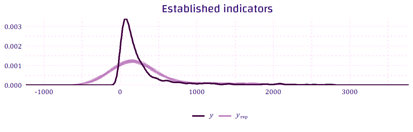
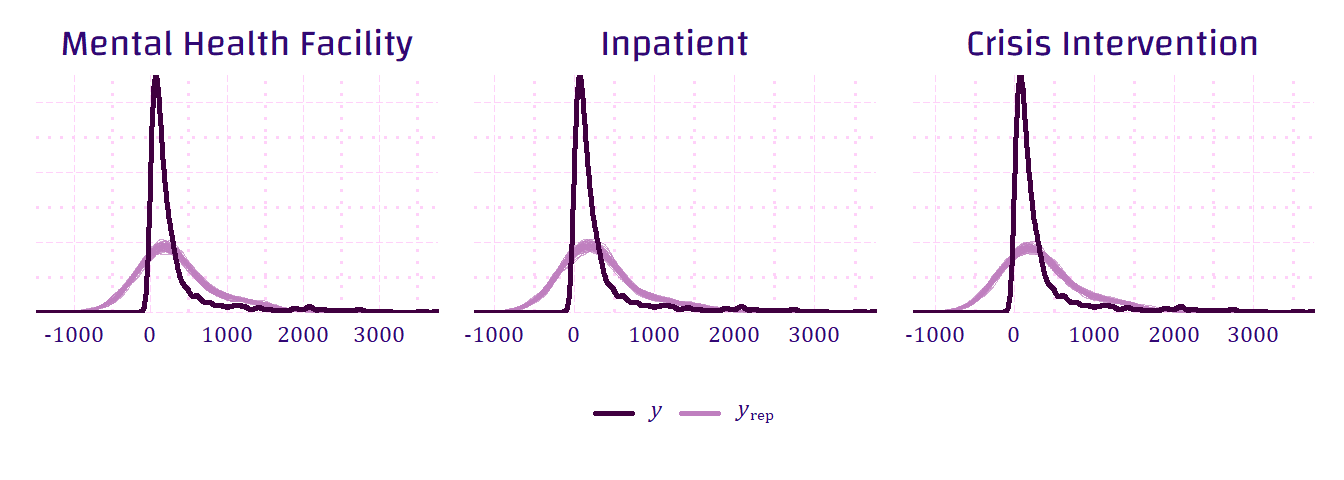
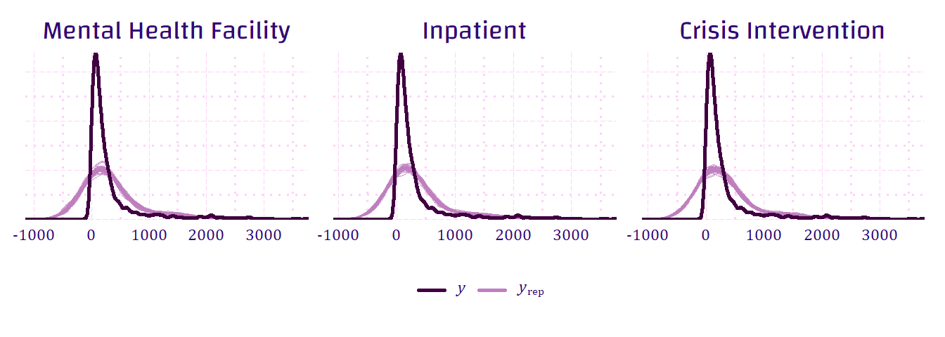
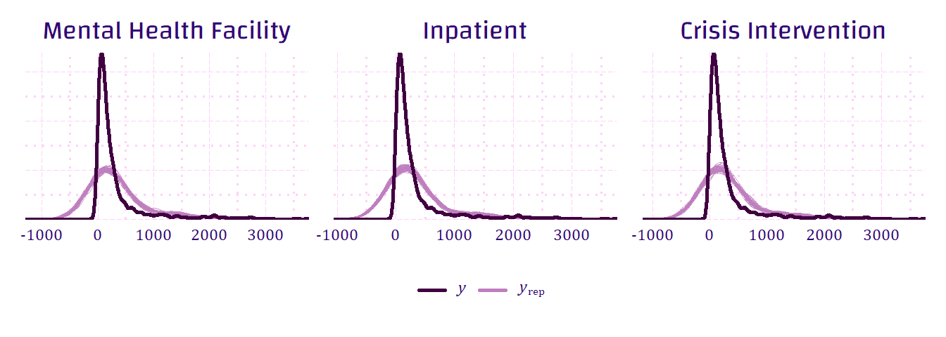
The following figures demonstrate the fit of the model with the original data. It does not appear to be a perfect fit because so many tracts had a rate of zero or close to zero rate of imprisonment, and a negative rate is not possible. Since the model can predict outcomes below zero, the fit is not perfect with a greater spread in the distribution around zero, as opposed to the high peak and drop in the original data.
Proximity to mental health facilities
\[ \begin{aligned} Y_{ij} | \beta_{0j}, \beta_5, \sigma_y \sim N(\mu_{ij}, \sigma_y^2) \;\; \text{ with } \;\; \mu_{ij} =& \beta_{0j} + \\ &\beta_5\text{Distance to Facility}_{ij}\\ \\ Y_{ij} | \beta_{0j}, \beta_4, \beta_5, \sigma_y \sim N(\mu_{ij}, \sigma_y^2) \;\; \text{ with } \;\; \mu_{ij} =& \beta_{0j} + \\ &\beta_4\text{Urban}_{ij} + \\ &\beta_5\text{Distance to Facility}_{ij} \\ \\ Y_{ij} | \beta_{0j}, \beta_1, \beta_2, \beta_3, \beta_4, \beta_5, \sigma_y \sim N(\mu_{ij}, \sigma_y^2) \;\; \text{ with } \;\; \mu_{ij} =& \beta_{0j} + \\ &\beta_1\text{Percent Black}_{ij} + \\ &\beta_2\text{Median Income}_{ij} + \\ &\beta_3\text{Unemployment Rate}_{ij} + \\ &\beta_4\text{Urban}_{ij} + \\ &\beta_5\text{Distance to Facility}_{ij} \\ \\ \beta_{0j} | \beta_0, \sigma_0 \stackrel{ind}{\sim} & N(\beta_0, \sigma_0^2) \\ \beta_{0c} \sim & N(100, 10^2) \\ \beta_1 \sim & N(100, 60) \\ \beta_2 \sim & N(-50, 15) \\ \beta_3 \sim & N(100, 25) \\ \beta_4 \sim & N(-100, 35) \\ \beta_5 \sim & N(100, 25) \\ \sigma \sim & \text{Exp}(l) \\ \sigma_y \sim & \text{Exp}(0.072) \\ \sigma_0 \sim & \text{Exp}(1) \\ \end{aligned} \]
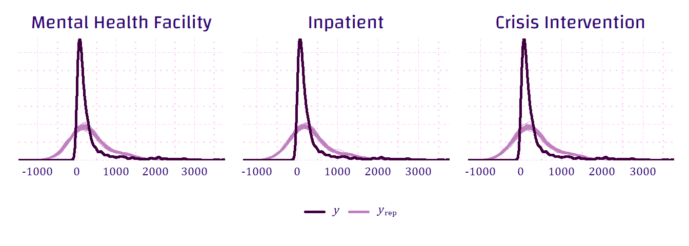
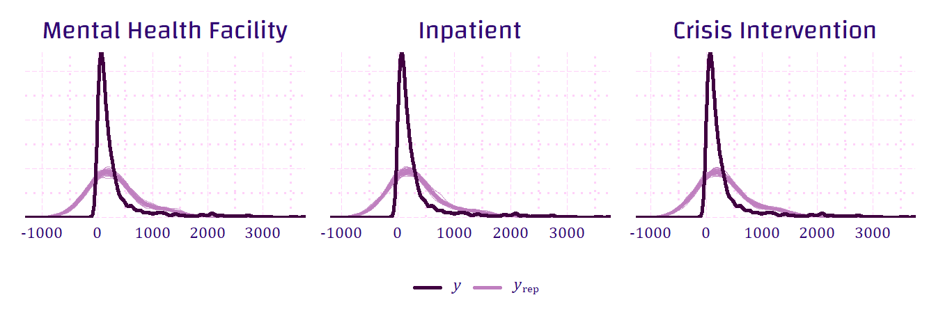
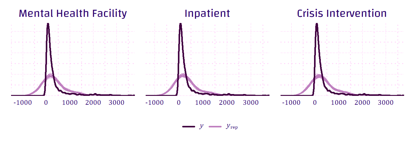
Since each tract has three variables regarding distance to facilities, three models for each equation were evaluated—distance to any mental health facility, distance to an inpatient mental health facility, and distance to an inpatient mental health facility with crisis intervention. The following figures demonstrate the fit of the model with the original data. It does not appear to be a perfect fit because so many tracts had a rate of zero or close to zero rate of imprisonment, and a negative rate is not possible. Since the model can predict outcomes below zero, the fit is not perfect with a greater spread in the distribution around zero, as opposed to the high peak and drop in the original data.
Distance to Mental Health Facilities
\[ \begin{aligned} Y_{ij} | \beta_{0j}, \beta_5, \sigma_y \sim N(\mu_{ij}, \sigma_y^2) \;\; \text{ with } \;\; \mu_{ij} =& \beta_{0j} + \beta_5\text{Distance to Facility}_{ij}\\ \end{aligned} \]
Distance to Mental Health Facilities and Urban/Rural Classification
\[ \begin{aligned} Y_{ij} | \beta_{0j}, \beta_4, \beta_5, \sigma_y \sim N(\mu_{ij}, \sigma_y^2) \;\; \text{ with } \;\; \mu_{ij} =& \beta_{0j} + \beta_4\text{Urban}_{ij} + \\ &\beta_5\text{Distance to Facility}_{ij} \\ \end{aligned} \]
Distance to Mental Health Facilities and All Other Variables
\[ \begin{aligned} Y_{ij} | \beta_{0j}, \beta_1, \beta_2, \beta_3, \beta_4, \beta_5, \sigma_y \sim N(\mu_{ij}, \sigma_y^2) \;\; \text{ with } \;\; \mu_{ij} =& \beta_{0j} + \\ &\beta_1\text{Percent Black}_{ij} + \\ &\beta_2\text{Median Income}_{ij} + \\ &\beta_3\text{Unemployment Rate}_{ij} + \\ &\beta_4\text{Urban}_{ij} + \\ &\beta_5\text{Distance to Facility}_{ij} \\ \end{aligned} \]
Code
Setup
knitr::opts_chunk$set(echo = FALSE,
                      include = TRUE,
                      message = FALSE,
                      warning = FALSE,
                      cache = TRUE)

library(tidyverse)
library(modelsummary)
library(scales)
library(readr)
library(tufte)
library(broom)
library(tinytex)
library(summarytools)
library(patchwork)
library(stringr)
library(ggpmisc)
library(cowplot)
library(grid)
library(ggridges)
library(bayesrules)
library(rstanarm)
library(rstan)
library(bayesplot)
library(tidybayes)
library(broom.mixed)
library(extrafont)
library(googlesheets4)
library(gt)
library(targets)
library(ggdag)
library(dagitty)
library(here)
library(pointblank)
library(lme4)
library(prismatic)
library(tidycensus)

colors <- c("#7400CC", "#CC0AA4", "#3ACC14", "#0E0ACC",
            "#0E0ACC", "#0ACCC5", "#CC1F14", "#1471CC",
            "#805713", "#4F008C", "#B785DD")
colors1 <- c("#CCAC14", "#CC1F14")
colors2 <- c("#0ACCC5", "#0E0ACC", "#0E0ACC")
colors3 <- c("#0ACCC5", "#7400CC", "#CC0AA4", "#3ACC14", "#0E0ACC")


pink4 <- c("#F3D9F9", "#DE9BD0", "#D656BB", "#B04585")
green3 <- c("#C3DEC8", "#6FD555", "#4D7D4A")
green5 <- c("#C3DEC8", "#A8DD9B", "#6FD555", "#4CB045", "#4D7D4A")

my_pct <- label_percent(accuracy = 0.1, scale = 1)
my_pct1 <- label_percent(accuracy = 0.1)
my_pct100 <- label_percent(accuracy = 1, scale = 1)
my_pct100_2 <- label_percent(accuracy = 1)
my_number <- label_number(accuracy = 1, big.mark = ",")
my_number1 <- label_number(accuracy = .01, big.mark = ",")
my_number2 <- label_number(accuracy = 1, suffix = " min")
my_number3 <- label_number(accuracy = .1)
my_dollar <- label_number(accuracy = 1, prefix = "$", big.mark = ",")

th_md <- theme_light() +
  theme(plot.title = element_text(family = "Changa",
                                  color = "#310873",
                                  size = 14,
                                  hjust = .5),
        plot.subtitle = element_text(family = "Changa",
                                     color = "#310873",
                                     size = 12,
                                     hjust = .5),
        plot.caption = element_text(family = "Cambria",
                                    color = "#310873",
                                    size = 8),
        axis.title = element_text(family = "Changa",
                                  color = "#310873"),
        axis.text = element_text(family = "Cambria",
                                 color = "#310873"),
        axis.ticks = element_blank(),
        strip.text = element_text(family = "Changa",
                                  color = "#310873",
                                  size = 12),
        strip.background = element_blank(),
        legend.text = element_text(family = "Cambria",
                                   color = "#310873"),
        legend.title = element_text(family = "Changa",
                                    color = "#310873"),
        legend.position = "bottom",
        panel.border = element_blank(),
        panel.grid.major = element_line(color = "#FFD1F9",
                                        linewidth = .35,
                                        linetype = "longdash"),
        panel.grid.minor = element_line(color = "#FFD1F9",
                                        linewidth = .6,
                                        linetype = "dotted"))

custom_labels <- function(x) {
  labels <- as.character(x)
  labels[1] <- paste0(labels[1], " min")
  return(labels)
}

pct <- function(x, page_width = 5.5) {
  if (knitr::pandoc_to("latex")) {
    paste0(page_width * (x / 100), "in")
  } else {
    gt::pct(x)
  }
}
th_md <- theme_light() + theme(panel.grid.major = element_line(color = “#FFD1F9”, linewidth = .5, linetype = “longdash”), panel.grid.minor = element_line(color = “#FFD1F9”, linewidth = .5, linetype = “dotted”), panel.border = element_blank(), axis.ticks = element_blank(), axis.text = element_text(family = “Cambria”), axis.title = element_text(family = “Changa”), plot.title = element_text(size = 14, family = “Changa”), plot.caption = element_text(family = “Cambria”), legend.text = element_text(family = “Changa”), legend.title = element_text(family = “Changa”))
## Data Manipulation in R

::: {.cell hash='prisoners_cache/html/facilities2_c4675a1de768bb3c8256546808227e8a'}

```{.r .cell-code}
## Extract facilities data from PDF.
## Parse data into a dataset with facility name, address, and services in Sheets.

MD <- readRDS("data/MD.RDS")
facilities <- read_csv("data/Facilities21.csv")

## Geocode facilities data in ArcGIS Pro.
## Join MD.csv to ACS tracts in ArcGIS for mapping.
## Join geocoded facilities with joined MD.csv and ACS tracts in ArcGIS Pro.
##
## Calculate distances to mental health facilities in ArcGIS Pro.
## Calculate distances to inpatient facilities in ArcGIS Pro.
## Calculate distances to inpatient facilities with Crisis Intervention in ArcGIS Pro.

## Load Calculated Distance Data
list_csv_files <- list.files(path = "data/gis/")
gis <- read_csv(paste0("data/gis/", list_csv_files), id = "file_name") %>%
  mutate(FIPS = as.numeric(substr(Name, 1, regexpr(" - ", Name) - 1))) %>%
  select(file_name, Name, FIPS, Total_TravelTime, Total_Miles)

## Miles to Nearest Mental Health Facility
mhf <- gis %>%
  filter(file_name == "data/gis/rural.csv" |
           file_name == "data/gis/urban.csv") %>%
  rename(miles2mhf = Total_Miles,
         tract2mhf = Name) %>%
  select(tract2mhf, FIPS, miles2mhf)

## Minutes to Nearest Mental Health Facility
mhf_time <- gis %>%
  filter(file_name == "data/gis/rural_time.csv" |
           file_name == "data/gis/urban_time.csv") %>%
  rename(time2mhf = Total_TravelTime,
         tract2mhf_time = Name) %>%
  select(tract2mhf_time, FIPS, time2mhf)

## Miles to Nearest Inpatient Mental Health Facility
hi <- gis %>%
  filter(file_name == "data/gis/rural_HI.csv" |
           file_name == "data/gis/urban_HI.csv") %>%
  rename(miles2inpatient = Total_Miles,
         tract2inpatient = Name) %>%
  select(tract2inpatient, FIPS, miles2inpatient)

## Minutes to Nearest Inpatient Mental Health Facility
hi_time <- gis %>%
  filter(file_name == "data/gis/rural_time_HI.csv" |
           file_name == "data/gis/urban_time_HI.csv") %>%
  rename(time2inpatient = Total_TravelTime,
         tract2inpatient_time = Name) %>%
  select(tract2inpatient_time, FIPS, time2inpatient)

## Miles to Nearest Inpatient Mental Health Facility with Crisis Intervention
crisis <- gis %>%
  filter(file_name == "data/gis/rural_crisis.csv" |
           file_name == "data/gis/urban_crisis.csv") %>%
  rename(miles2crisis = Total_Miles,
         tract2crisis = Name) %>%
  select(tract2crisis, FIPS, miles2crisis)

## Minutes to Nearest Inpatient Mental Health Facility with Crisis Intervention
crisis_time <- gis %>%
  filter(file_name == "data/gis/rural_time_crisis.csv" |
           file_name == "data/gis/urban_time_crisis.csv") %>%
  rename(time2crisis = Total_TravelTime,
         tract2crisis_time = Name) %>%
  select(tract2crisis_time, FIPS, time2crisis)
:::
## Rural housing counts from census
rural <- get_decennial(geography = "tract",
                       variables = "H2_003N",
                       summary_var = "H2_001N",
                       state = 24,
                       year = 2020,
                       sumfile = "dhc") %>%
  mutate(pctRural = (value / summary_value) * 100) %>%
  rename(FIPS = GEOID) %>%
  select(FIPS, pctRural) %>%
  mutate(urban = ifelse(pctRural == 0, 1, 0),
         urban_cat = ifelse(pctRural == 0, "Urban", "Rural"))

## Other variables from ACS
acsMD <- get_acs(geography = "tract",
                 variables = c(IncomeMedian = "S1901_C02_012",
                               Total_Pop = "S0701_C01_001",
                               black_pop = "S0701_C01_016",
                               povStatusDet = "S0701_C01_049",
                               underPov = "S0701_C01_050",
                               UnempRate16 = "S2301_C04_001"),
                 state = "MD",
                 year = 2020) %>%
  spread(variable, estimate) %>%
  group_by(GEOID, NAME) %>%
  summarize(IncomeMedian = sum(IncomeMedian, na.rm = TRUE),
            Total_Pop = sum(Total_Pop, na.rm = TRUE),
            black_pop = sum(black_pop, na.rm = TRUE),
            povStatusDet = sum(povStatusDet, na.rm = TRUE),
            underPov = sum(underPov, na.rm = TRUE),
            UnempRate16 = sum(UnempRate16, na.rm = TRUE)) %>%
  rename(FIPS = GEOID) %>%
  merge(rural, by = "FIPS")
## Load Imprisonment Data
MD <- read_csv("data/Imprisonment_rates.csv") %>%
select(FIPS, Imprisonment_Rate) %>%
merge(acsMD, by = "FIPS") %>% ## Merge with ACS data
mutate(tract = substr(NAME, 1, regexpr(",", NAME) - 1)) %>%
mutate(County = substr(NAME,
regexpr(",", NAME) + 2,
regexpr("County", NAME) + 5),
County = ifelse(str_detect(NAME, "Baltimore city"),
"Baltimore City",
trimws(County, which = c("both")))) %>% ## Extract County Column
mutate(pctBlack = (black_pop / Total_Pop) * 100,
pctUnderPoverty = (underPov / povStatusDet) * 100) %>% ## Calculate Percentages
mutate(black = case_when(pctBlack > 50 ~ 1,
pctBlack <= 50 ~ 0),
black_cat = factor(black,
labels = c("Not Majority Black Tracts",
"Majority Black Tracts"))) %>% ## Create dummies
left_join(mhf, by = "FIPS") %>%
left_join(mhf_time, by = "FIPS") %>%
left_join(hi, by = "FIPS") %>%
left_join(hi_time, by = "FIPS") %>%
left_join(crisis, by = "FIPS") %>%
left_join(crisis_time, by = "FIPS")
## Save data
saveRDS(MD, file = "data/MD_GIS_raw.RDS")
write.csv(MD, "data/MD_GIS_raw.csv", row.names=FALSE)MD <- readRDS("data/MD_GIS_raw.RDS")
zeros <- MD %>%
filter(Imprisonment_Rate == 0)
# Interpolating erroneous zeros for IncomeMedian
estincome24003706404 <- (((195588 + 146607 +
94985 + 92557 +
101167) / 5) + # Adjacent tracts
119426.503937) / 2 # County median
estincome24021750801 <- (((75868 + 135163 +
112527 + 56250 +
124625 + 99257 +
114757) / 7) + # Adjacent tracts
113061.553846154) / 2 # County median
estincome24045010503 <- (((61525 + 37000 +
102244 + 80089 +
110536 + 58256) / 6) + # Adjacent tracts
68801.0476190476) / 2 # County median
estincomeBmore1 <- (((77679 + 128969 +
88463 + 15114 +
43359 + 21222 +
59643 + 65156 +
41398 + 162578 +
24274) / 11) + # Adjacent tracts
71972.8172588833) / 2 # County median
estincomeBmore2 <- (((134708 + 154018 +
80250 + 50513 +
26521 + 77188) / 6) +
71972.8172588833) / 2 # County median
estincomeBmore3 <- (((66387 + 50490 + 52059) / 3) + # Adjacent tracts
(71972.8172588833 +
(119426.503937008 * 3)) / 4) / 2 # County medians
MD <- MD %>%
filter(Total_Pop >= 100, ## Drop Tracts with a population below 100
# Corrections
FIPS != 24510100300, # Baltimore jail
FIPS != 24043011000, # Maryland correctional training center
FIPS != 24003740400, # Maryland State Prison
# Campuses
FIPS != 24005403801, # Stevenson University Greenspring Campus
FIPS != 24005490605, # Towson University
FIPS != 24510271300, # St Mary's Seminary & University
FIPS != 24031700836, # Research park
FIPS != 24033980000, # University of Maryland
FIPS != 24005492500, # University of Maryland
# Military
FIPS != 24017850201, # Naval Support Facility Indian Head /
# Smallwood State Park
FIPS != 24003706700, # United States Naval Academy
FIPS != 24003740601, # Fort George G. Meade
FIPS != 24003740602, # Fort George G. Meade
FIPS != 24021751203, # AFMESA ???
FIPS != 24025303102, # Churchville Test Area
FIPS != 24025306500, # Army Pulse Radiation Facility
FIPS != 24031705000, # National Institutes of Health /
# Walter Reed National Military Medical Center
FIPS != 24033801105, # Joint Base Andrews
FIPS != 24033801106, # Joint Base Andrews
# Protected Land
FIPS != 24005400500, # Patapsco Valley State Park - Hilton Area
FIPS != 24013505206, # Patapsco Valley State Park- McKeldin Area
FIPS != 24027601104, # Patapsco Valley State Park - Hilton Area /
# Rockburn Branch Park
FIPS != 24031700606, # Muddy Branch Greenway Trail
FIPS != 24005408502, # Loch Raven Reservoir
FIPS != 24031701210, # Rock Creek Regional Park
FIPS != 24031701219, # Parklawn Community Garden
FIPS != 24031706012, # Cabin John Regional Park
FIPS != 24031700209, # Goshen Recreational Park /
# Damascus Recreational Park
# Other
FIPS != 24001001300, # Allegany County Fairgrounds
FIPS != 24031702502, # Commercial only
FIPS != 24031704403, # Commercial only
FIPS != 24031702603, # Commercial only
FIPS != 24031704805, # Bethesda Chevy Chase High School /
# Commercial only
) %>%
mutate(IncomeMedian = case_when(FIPS == 24003706404 ~ estincome24003706404,
FIPS == 24021750801 ~ estincome24021750801,
FIPS == 24045010503 ~ estincome24045010503,
FIPS == 24510040200 ~ estincomeBmore1,
FIPS == 24510170100 ~ estincomeBmore1,
FIPS == 24510170200 ~ estincomeBmore1,
FIPS == 24510170300 ~ estincomeBmore1,
FIPS == 24510180300 ~ estincomeBmore1,
FIPS == 24510060100 ~ estincomeBmore2,
FIPS == 24510250402 ~ estincomeBmore3,
TRUE ~ IncomeMedian)) %>% # Interpolate erroneous zeros
mutate(IncomeMedian1000 = IncomeMedian / 1000) %>% ## Scale median income by 1000
mutate(County = substr(NAME,
regexpr(",", NAME) + 2,
regexpr("County", NAME) + 5),
County = ifelse(str_detect(NAME, "Baltimore city"),
"Baltimore City",
trimws(County, which = c("both")))) ## Extract County Column
## Save data
saveRDS(MD, file = "data/MD_GIS.RDS")
write.csv(MD, "data/MD_GIS.csv", row.names=FALSE)MD <- readRDS("data/MD_GIS.RDS")
## Aggregate to the County Level
MD_counties <- MD %>%
select(FIPS, NAME, County, Imprisonment_Rate, Total_Pop, IncomeMedian,
pctBlack, pctUnderPoverty, UnempRate16, pctRural) %>%
group_by(County) %>%
summarise(Imprisonment_RateCounty = mean(Imprisonment_Rate),
Total_PopCounty = sum(Total_Pop),
IncomeMedianCounty = mean(IncomeMedian),
pctBlackCounty = mean(pctBlack),
pctUnderPovertyCounty = mean(pctUnderPoverty),
UnempRate16County = mean(UnempRate16),
pctRuralCounty = mean(pctRural)) %>%
mutate(ruralCounty = ifelse(pctRuralCounty > 20, TRUE, FALSE))
MD <- MD %>%
merge(MD_counties, by = "County")
## Save data
saveRDS(MD, file = "data/MD.RDS")
saveRDS(MD_counties, file = "data/MD_counties.RDS")
write.csv(MD_counties, "data/MD_counties.csv", row.names=FALSE)
write.csv(MD, "data/MD.csv", row.names=FALSE)Modeling Code
if (file.exists("data/alldemos.rds")) {
  alldemos_ <- readRDS("data/alldemos.rds")
} else {
  alldemos_ <- stan_glmer(Imprisonment_Rate ~ pctBlack +
                                              IncomeMedian1000 +
                                              UnempRate16 +
                                              urban +
                                              (1 + IncomeMedian1000 | County),
                          data = MD,
                          family = gaussian,
                          chains = 4, iter = 5000*2, seed = 84735,
                          cores = 4)

  saveRDS(alldemos_, "data/alldemos.rds")
}

color_scheme_set("purple")
ppc_dens_overlay(y = MD$Imprisonment_Rate,
                 yrep = posterior_predict(alldemos_,
                                          draws = 50)) +
  th_md

all <- alldemos_ %>%
  spread_draws(pctBlack, IncomeMedian1000, UnempRate16, urban) %>%
  summarize(pctBlack_greater_0 = sum(pctBlack > 0) / n(),
            IncomeMedian_greater_0 = sum(IncomeMedian1000 > 0) / n(),
            Unemp_greater_0 = sum(UnempRate16 > 0) / n(),
            urban_greater_0 = sum(urban > 0) / n())

all_ <- alldemos_ %>%
  spread_draws(pctBlack, IncomeMedian1000, UnempRate16, urban) %>%
  median_hdi()

all_u <- alldemos_ %>%
  spread_draws(urban) %>%
  median_hdi(.width = .80)
Distance to Mental Health Facilities with Crisis Intervention
if (file.exists("data/distance_mh.rds")) {
  distance_mh <- readRDS("data/distance_mh.rds")
} else {
  distance_mh <- stan_glmer(Imprisonment_Rate ~ miles2mhf +
                              (1 + miles2mhf | County),
                            data = MD,
                            family = gaussian,
                            chains = 4, iter = 5000*2, seed = 84735,
                            cores = 4)

  saveRDS(distance_mh, "data/distance_mh.rds")
}

color_scheme_set("purple")
dmh <- ppc_dens_overlay(y = MD$Imprisonment_Rate,
                        yrep = posterior_predict(distance_mh,
                                                 draws = 50)) +
  labs(title = "Mental Health Facility") +
  th_md +
  theme(axis.text.y = element_blank())

if (file.exists("data/distance_inpatient.rds")) {
  distance_inpatient <- readRDS("data/distance_inpatient.rds")
} else {
  distance_inpatient <- stan_glmer(Imprisonment_Rate ~ miles2inpatient +
                                     (1 + miles2inpatient | County),
                                   data = MD,
                                   family = gaussian,
                                   chains = 4, iter = 5000*2, seed = 84735,
                                   cores = 4)

  saveRDS(distance_inpatient, "data/distance_inpatient.rds")
}

color_scheme_set("purple")
di <- ppc_dens_overlay(y = MD$Imprisonment_Rate,
                       yrep = posterior_predict(distance_inpatient,
                                                draws = 50)) +
  labs(title = "Inpatient") +
  th_md +
  theme(axis.text.y = element_blank())

if (file.exists("data/distance_crisis.rds")) {
  distance_crisis <- readRDS("data/distance_crisis.rds")
} else {
  distance_crisis <- stan_glmer(Imprisonment_Rate ~ miles2crisis +
                                  (1 + miles2crisis | County),
                                data = MD,
                                family = gaussian,
                                chains = 4, iter = 5000*2, seed = 84735,
                                cores = 4)

  saveRDS(distance_crisis, "data/distance_crisis.rds")
}

color_scheme_set("purple")
dcr <- ppc_dens_overlay(y = MD$Imprisonment_Rate,
                        yrep = posterior_predict(distance_crisis,
                                                 draws = 50)) +
  labs(title = "Crisis Intervention") +
  th_md +
  theme(axis.text.y = element_blank())

dmh + di + dcr +
  plot_layout(guides = "collect") &
  theme(legend.position = "bottom")

dist_mh <- distance_mh %>%
  spread_draws(miles2mhf) %>%
  summarize(miles2mhf_greater_0 = sum(miles2mhf > 0) / n())

dist_mh_ <- distance_mh %>%
  spread_draws(miles2mhf) %>%
  median_hdi()

dist_inpatient <- distance_inpatient %>%
  spread_draws(miles2inpatient) %>%
  summarize(miles2inpatient_greater_0 = sum(miles2inpatient > 0) / n())

dist_inpatient_ <- distance_inpatient %>%
  spread_draws(miles2inpatient) %>%
  median_hdi()

dist_crisis <- distance_crisis %>%
  spread_draws(miles2crisis) %>%
  summarize(miles2crisis_greater_0 = sum(miles2crisis > 0) / n())

dist_crisis_ <- distance_crisis %>%
  spread_draws(miles2crisis) %>%
  median_hdi()
if (file.exists("data/time_mh.rds")) {
time_mh <- readRDS("data/time_mh.rds")
} else {
time_mh <- stan_glmer(Imprisonment_Rate ~ time2mhf +
(1 + time2mhf | County),
data = MD,
family = gaussian,
chains = 4, iter = 5000*2, seed = 84735,
cores = 4)
saveRDS(time_mh, "data/time_mh.rds")
}
color_scheme_set("purple")
dmh <- ppc_dens_overlay(y = MD$Imprisonment_Rate,
yrep = posterior_predict(time_mh,
draws = 50)) +
labs(title = "Mental Health Facility") +
th_md +
theme(axis.text.y = element_blank())
if (file.exists("data/time_inpatient.rds")) {
time_inpatient <- readRDS("data/time_inpatient.rds")
} else {
time_inpatient <- stan_glmer(Imprisonment_Rate ~ time2inpatient +
(1 + time2inpatient | County),
data = MD,
family = gaussian,
chains = 4, iter = 5000*2, seed = 84735,
cores = 4)
saveRDS(time_inpatient, "data/time_inpatient.rds")
}
color_scheme_set("purple")
di <- ppc_dens_overlay(y = MD$Imprisonment_Rate,
yrep = posterior_predict(time_inpatient,
draws = 50)) +
labs(title = "Inpatient") +
th_md +
theme(axis.text.y = element_blank())
if (file.exists("data/time_crisis.rds")) {
time_crisis <- readRDS("data/time_crisis.rds")
} else {
time_crisis <- stan_glmer(Imprisonment_Rate ~ time2crisis +
(1 + time2crisis | County),
data = MD,
family = gaussian,
chains = 4, iter = 5000*2, seed = 84735,
cores = 4)
saveRDS(time_crisis, "data/time_crisis.rds")
}
color_scheme_set("purple")
dcr <- ppc_dens_overlay(y = MD$Imprisonment_Rate,
yrep = posterior_predict(time_crisis,
draws = 50)) +
labs(title = "Crisis Intervention") +
th_md +
theme(axis.text.y = element_blank())
dmh + di + dcr +
plot_layout(guides = "collect") &
theme(legend.position = "bottom")
ti_mh <- time_mh %>%
spread_draws(time2mhf) %>%
summarize(time2mhf_greater_0 = sum(time2mhf > 0) / n())
ti_mh_ <- time_mh %>%
spread_draws(time2mhf) %>%
median_hdi()
ti_inpatient <- time_inpatient %>%
spread_draws(time2inpatient) %>%
summarize(time2inpatient_greater_0 = sum(time2inpatient > 0) / n())
ti_inpatient_ <- time_inpatient %>%
spread_draws(time2inpatient) %>%
median_hdi()
ti_crisis <- time_crisis %>%
spread_draws(time2crisis) %>%
summarize(time2crisis_greater_0 = sum(time2crisis > 0) / n())
ti_crisis_ <- time_crisis %>%
spread_draws(time2crisis) %>%
median_hdi()Distance to Mental Health Facilities with Crisis Intervention and Urban/Rural Classification
if (file.exists("data/distance_rural_mh.rds")) {
  distance_rural_mh <- readRDS("data/distance_rural_mh.rds")
} else {
  distance_rural_mh <- stan_glmer(Imprisonment_Rate ~ miles2mhf +
                                    urban +
                                    (1 + miles2mhf | County),
                                  data = MD,
                                  family = gaussian,
                                  chains = 4, iter = 5000*2, seed = 84735,
                                  cores = 4)

  saveRDS(distance_rural_mh, "data/distance_rural_mh.rds")
}

color_scheme_set("purple")
drmh <- ppc_dens_overlay(y = MD$Imprisonment_Rate,
                         yrep = posterior_predict(distance_rural_mh,
                                                  draws = 50)) +
  labs(title = "Mental Health Facility") +
  th_md +
  theme(axis.text.y = element_blank())

if (file.exists("data/distance_rural_inpatient.rds")) {
  distance_rural_inpatient <- readRDS("data/distance_rural_inpatient.rds")
} else {
  distance_rural_inpatient <- stan_glmer(Imprisonment_Rate ~ miles2inpatient +
                                           urban +
                                           (1 + miles2inpatient | County),
                                         data = MD,
                                         family = gaussian,
                                         chains = 4, iter = 5000*2, seed = 84735,
                                         cores = 4)

  saveRDS(distance_rural_inpatient, "data/distance_rural_inpatient.rds")
}

color_scheme_set("purple")
dri <- ppc_dens_overlay(y = MD$Imprisonment_Rate,
                        yrep = posterior_predict(distance_rural_inpatient,
                                                 draws = 50)) +
  labs(title = "Inpatient") +
  th_md +
  theme(axis.text.y = element_blank())

if (file.exists("data/distance_rural_crisis.rds")) {
  distance_rural_crisis <- readRDS("data/distance_rural_crisis.rds")
} else {
  distance_rural_crisis <- stan_glmer(Imprisonment_Rate ~ miles2crisis +
                                        urban +
                                        (1 + miles2crisis | County),
                                      data = MD,
                                      family = gaussian,
                                      chains = 4, iter = 5000*2, seed = 84735,
                                      cores = 4)

  saveRDS(distance_rural_crisis, "data/distance_rural_crisis.rds")
}

color_scheme_set("purple")
drc <- ppc_dens_overlay(y = MD$Imprisonment_Rate,
                        yrep = posterior_predict(distance_rural_crisis,
                                                 draws = 50)) +
  labs(title = "Crisis Intervention") +
  th_md +
  theme(axis.text.y = element_blank())

drmh + dri + drc +
  plot_layout(guides = "collect") &
  theme(legend.position = "bottom")


dist_rural_mh <- distance_rural_mh %>%
  spread_draws(miles2mhf, urban) %>%
  summarize(miles2mhf_greater_0 = sum(miles2mhf > 0) / n(),
            urban_greater_0 = sum(urban > 0) / n())

dist_rural_mh_ <- distance_rural_mh %>%
  spread_draws(miles2mhf, urban) %>%
  median_hdi()

dist_rural_inpatient <- distance_rural_inpatient %>%
  spread_draws(miles2inpatient, urban) %>%
  summarize(miles2inpatient_greater_0 = sum(miles2inpatient > 0) / n(),
            urban_greater_0 = sum(urban > 0) / n())

dist_rural_inpatient_ <- distance_rural_inpatient %>%
  spread_draws(miles2inpatient, urban) %>%
  median_hdi()

dist_rural_crisis <- distance_rural_crisis %>%
  spread_draws(miles2crisis, urban) %>%
  summarize(miles2crisis_greater_0 = sum(miles2crisis > 0) / n(),
            urban_greater_0 = sum(urban > 0) / n())

dist_rural_crisis_ <- distance_rural_crisis %>%
  spread_draws(miles2crisis, urban) %>%
  median_hdi()
if (file.exists("data/time_rural_mh.rds")) {
time_rural_mh <- readRDS("data/time_rural_mh.rds")
} else {
time_rural_mh <- stan_glmer(Imprisonment_Rate ~ time2mhf +
urban +
(1 + time2mhf | County),
data = MD,
family = gaussian,
chains = 4, iter = 5000*2, seed = 84735,
cores = 4)
saveRDS(time_rural_mh, "data/time_rural_mh.rds")
}
color_scheme_set("purple")
drmh <- ppc_dens_overlay(y = MD$Imprisonment_Rate,
yrep = posterior_predict(time_rural_mh,
draws = 50)) +
labs(title = "Mental Health Facility") +
th_md +
theme(axis.text.y = element_blank())
if (file.exists("data/time_rural_inpatient.rds")) {
time_rural_inpatient <- readRDS("data/time_rural_inpatient.rds")
} else {
time_rural_inpatient <- stan_glmer(Imprisonment_Rate ~ time2inpatient +
urban +
(1 + time2inpatient | County),
data = MD,
family = gaussian,
chains = 4, iter = 5000*2, seed = 84735,
cores = 4)
saveRDS(time_rural_inpatient, "data/time_rural_inpatient.rds")
}
color_scheme_set("purple")
dri <- ppc_dens_overlay(y = MD$Imprisonment_Rate,
yrep = posterior_predict(time_rural_inpatient,
draws = 50)) +
labs(title = "Inpatient") +
th_md +
theme(axis.text.y = element_blank())
if (file.exists("data/time_rural_crisis.rds")) {
time_rural_crisis <- readRDS("data/time_rural_crisis.rds")
} else {
time_rural_crisis <- stan_glmer(Imprisonment_Rate ~ time2crisis +
urban +
(1 + time2crisis | County),
data = MD,
family = gaussian,
chains = 4, iter = 5000*2, seed = 84735,
cores = 4)
saveRDS(time_rural_crisis, "data/time_rural_crisis.rds")
}
color_scheme_set("purple")
drc <- ppc_dens_overlay(y = MD$Imprisonment_Rate,
yrep = posterior_predict(time_rural_crisis,
draws = 50)) +
labs(title = "Crisis Intervention") +
th_md +
theme(axis.text.y = element_blank())
drmh + dri + drc +
plot_layout(guides = "collect") &
theme(legend.position = "bottom")
ti_rural_mh <- time_rural_mh %>%
spread_draws(time2mhf, urban) %>%
summarize(time2mhf_greater_0 = sum(time2mhf > 0) / n(),
urban_greater_0 = sum(urban > 0) / n())
ti_rural_mh_ <- time_rural_mh %>%
spread_draws(time2mhf, urban) %>%
median_hdi()
ti_rural_inpatient <- time_rural_inpatient %>%
spread_draws(time2inpatient, urban) %>%
summarize(time2inpatient_greater_0 = sum(time2inpatient > 0) / n(),
urban_greater_0 = sum(urban > 0) / n())
ti_rural_inpatient_ <- time_rural_inpatient %>%
spread_draws(time2inpatient, urban) %>%
median_hdi()
ti_rural_crisis <- time_rural_crisis %>%
spread_draws(time2crisis, urban) %>%
summarize(time2crisis_greater_0 = sum(time2crisis > 0) / n(),
urban_greater_0 = sum(urban > 0) / n())
ti_rural_crisis_ <- time_rural_crisis %>%
spread_draws(time2crisis, urban) %>%
median_hdi()Distance to Mental Health Facilities with Crisis Intervention and All Other Variables
if (file.exists("data/distance_all_mh.rds")) {
  distance_all_mh <- readRDS("data/distance_all_mh.rds")
} else {
  distance_all_mh <- stan_glmer(Imprisonment_Rate ~ miles2mhf +
                                                    pctBlack +
                                                    IncomeMedian1000 +
                                                    UnempRate16 +
                                                    urban +
                                                    (1 + miles2mhf | County),
                             data = MD,
                             family = gaussian,
                             chains = 4, iter = 5000*2, seed = 84735,
                             cores = 4)

  saveRDS(distance_all_mh, "data/distance_all_mh.rds")
}

color_scheme_set("purple")
damh <- ppc_dens_overlay(y = MD$Imprisonment_Rate,
                         yrep = posterior_predict(distance_all_mh,
                                                  draws = 50)) +
  labs(title = "Mental Health Facility") +
  th_md +
  theme(axis.text.y = element_blank())

if (file.exists("data/distance_all_inpatient.rds")) {
  distance_all_inpatient <- readRDS("data/distance_all_inpatient.rds")
} else {
  distance_all_inpatient <- stan_glmer(Imprisonment_Rate ~ miles2inpatient +
                                                           pctBlack +
                                                           IncomeMedian1000 +
                                                           UnempRate16 +
                                                           urban +
                                                           (1 + miles2inpatient | County),
                             data = MD,
                             family = gaussian,
                             chains = 4, iter = 5000*2, seed = 84735,
                             cores = 4)

  saveRDS(distance_all_inpatient, "data/distance_all_inpatient.rds")
}

color_scheme_set("purple")
dai <- ppc_dens_overlay(y = MD$Imprisonment_Rate,
                        yrep = posterior_predict(distance_all_inpatient,
                                                 draws = 50)) +
  labs(title = "Inpatient") +
  th_md +
  theme(axis.text.y = element_blank())

if (file.exists("data/distance_all_crisis.rds")) {
  distance_all_crisis <- readRDS("data/distance_all_crisis.rds")
} else {
  distance_all_crisis <- stan_glmer(Imprisonment_Rate ~ miles2crisis +
                                                        pctBlack +
                                                        IncomeMedian1000 +
                                                        UnempRate16 +
                                                        urban +
                                                        (1 + miles2crisis | County),
                             data = MD,
                             family = gaussian,
                             chains = 4, iter = 5000*2, seed = 84735,
                             cores = 4)

  saveRDS(distance_all_crisis, "data/distance_all_crisis.rds")
}

color_scheme_set("purple")
dac <- ppc_dens_overlay(y = MD$Imprisonment_Rate,
                        yrep = posterior_predict(distance_all_crisis,
                                                 draws = 50)) +
  labs(title = "Crisis Intervention") +
  th_md +
  theme(axis.text.y = element_blank())

damh + dai + dac +
  plot_layout(guides = "collect") &
  theme(legend.position = "bottom")


dist_all_mh <- distance_all_mh %>%
  spread_draws(miles2mhf, pctBlack, IncomeMedian1000, UnempRate16, urban) %>%
  summarize(miles2mhf_greater_0 = sum(miles2mhf > 0) / n(),
            pctBlack_greater_0 = sum(pctBlack > 0) / n(),
            IncomeMedian_greater_0 = sum(IncomeMedian1000 > 0) / n(),
            Unemp_greater_0 = sum(UnempRate16 > 0) / n(),
            urban_greater_0 = sum(urban > 0) / n())

dist_all_mh_ <- distance_all_mh %>%
  spread_draws(miles2mhf, pctBlack, IncomeMedian1000, UnempRate16, urban) %>%
  median_hdi()

dist_all_inpatient <- distance_all_inpatient %>%
  spread_draws(miles2inpatient, pctBlack, IncomeMedian1000, UnempRate16, urban) %>%
  summarize(miles2inpatient_greater_0 = sum(miles2inpatient > 0) / n(),
            pctBlack_greater_0 = sum(pctBlack > 0) / n(),
            IncomeMedian_greater_0 = sum(IncomeMedian1000 > 0) / n(),
            Unemp_greater_0 = sum(UnempRate16 > 0) / n(),
            urban_greater_0 = sum(urban > 0) / n())

dist_all_inpatient_ <- distance_all_inpatient %>%
  spread_draws(miles2inpatient, pctBlack, IncomeMedian1000, UnempRate16, urban) %>%
  median_hdi()

dist_all_crisis <- distance_all_crisis %>%
  spread_draws(miles2crisis, pctBlack, IncomeMedian1000, UnempRate16, urban) %>%
  summarize(miles2crisis_greater_0 = sum(miles2crisis > 0) / n(),
            pctBlack_greater_0 = sum(pctBlack > 0) / n(),
            IncomeMedian_greater_0 = sum(IncomeMedian1000 > 0) / n(),
            Unemp_greater_0 = sum(UnempRate16 > 0) / n(),
            urban_greater_0 = sum(urban > 0) / n())

dist_all_crisis_ <- distance_all_crisis %>%
  spread_draws(miles2crisis, pctBlack, IncomeMedian1000, UnempRate16, urban) %>%
  median_hdi()
if (file.exists("data/time_all_mh.rds")) {
time_all_mh <- readRDS("data/time_all_mh.rds")
} else {
time_all_mh <- stan_glmer(Imprisonment_Rate ~ time2mhf +
pctBlack +
IncomeMedian1000 +
UnempRate16 +
urban +
(1 + time2mhf | County),
data = MD,
family = gaussian,
chains = 4, iter = 5000*2, seed = 84735,
cores = 4)
saveRDS(time_all_mh, "data/time_all_mh.rds")
}
color_scheme_set("purple")
damh <- ppc_dens_overlay(y = MD$Imprisonment_Rate,
yrep = posterior_predict(time_all_mh,
draws = 50)) +
labs(title = "Mental Health Facility") +
th_md +
theme(axis.text.y = element_blank())
if (file.exists("data/time_all_inpatient.rds")) {
time_all_inpatient <- readRDS("data/time_all_inpatient.rds")
} else {
time_all_inpatient <- stan_glmer(Imprisonment_Rate ~ time2inpatient +
pctBlack +
IncomeMedian1000 +
UnempRate16 +
urban +
(1 + time2inpatient | County),
data = MD,
family = gaussian,
chains = 4, iter = 5000*2, seed = 84735,
cores = 4)
saveRDS(time_all_inpatient, "data/time_all_inpatient.rds")
}
color_scheme_set("purple")
dai <- ppc_dens_overlay(y = MD$Imprisonment_Rate,
yrep = posterior_predict(time_all_inpatient,
draws = 50)) +
labs(title = "Inpatient") +
th_md +
theme(axis.text.y = element_blank())
if (file.exists("data/time_all_crisis.rds")) {
time_all_crisis <- readRDS("data/time_all_crisis.rds")
} else {
time_all_crisis <- stan_glmer(Imprisonment_Rate ~ time2crisis +
pctBlack +
IncomeMedian1000 +
UnempRate16 +
urban +
(1 + time2crisis | County),
data = MD,
family = gaussian,
chains = 4, iter = 5000*2, seed = 84735,
cores = 4)
saveRDS(time_all_crisis, "data/time_all_crisis.rds")
}
color_scheme_set("purple")
dac <- ppc_dens_overlay(y = MD$Imprisonment_Rate,
yrep = posterior_predict(time_all_crisis,
draws = 50)) +
labs(title = "Crisis Intervention") +
th_md +
theme(axis.text.y = element_blank())
damh + dai + dac +
plot_layout(guides = "collect") &
theme(legend.position = "bottom")
ti_all_mh <- time_all_mh %>%
spread_draws(time2mhf, pctBlack, IncomeMedian1000, UnempRate16, urban) %>%
summarize(time2mhf_greater_0 = sum(time2mhf > 0) / n(),
pctBlack_greater_0 = sum(pctBlack > 0) / n(),
IncomeMedian_greater_0 = sum(IncomeMedian1000 > 0) / n(),
Unemp_greater_0 = sum(UnempRate16 > 0) / n(),
urban_greater_0 = sum(urban > 0) / n())
ti_all_mh_ <- time_all_mh %>%
spread_draws(time2mhf, pctBlack, IncomeMedian1000, UnempRate16, urban) %>%
median_hdi()
ti_all_inpatient <- time_all_inpatient %>%
spread_draws(time2inpatient, pctBlack, IncomeMedian1000, UnempRate16, urban) %>%
summarize(time2inpatient_greater_0 = sum(time2inpatient > 0) / n(),
pctBlack_greater_0 = sum(pctBlack > 0) / n(),
IncomeMedian_greater_0 = sum(IncomeMedian1000 > 0) / n(),
Unemp_greater_0 = sum(UnempRate16 > 0) / n(),
urban_greater_0 = sum(urban > 0) / n())
ti_all_inpatient_ <- time_all_inpatient %>%
spread_draws(time2inpatient, pctBlack, IncomeMedian1000, UnempRate16, urban) %>%
median_hdi()
ti_all_crisis <- time_all_crisis %>%
spread_draws(time2crisis, pctBlack, IncomeMedian1000, UnempRate16, urban) %>%
summarize(time2crisis_greater_0 = sum(time2crisis > 0) / n(),
pctBlack_greater_0 = sum(pctBlack > 0) / n(),
IncomeMedian_greater_0 = sum(IncomeMedian1000 > 0) / n(),
Unemp_greater_0 = sum(UnempRate16 > 0) / n(),
urban_greater_0 = sum(urban > 0) / n())
ti_all_crisis_ <- time_all_crisis %>%
spread_draws(time2crisis, pctBlack, IncomeMedian1000, UnempRate16, urban) %>%
median_hdi()Graphics
dag <- dagitty('
dag {
"`Median Income`" [adjusted,pos="1.5,1"]
"`% with Disability`" [pos="4.2,1"]
"`% Under Poverty`" [pos="3.4,1.0475"]
"`Unemployment`" [adjusted,pos="1,1.35"]
"`% Black`" [adjusted,pos="1.55,1.45"]
"`Urban/Rural Classification`" [adjusted,pos="2.25,1.55"]
"`% w/o Internet`" [pos="2.7,1.118"]
"`% w/o Health Insurance`" [pos="1.775,1.175"]
"`Access to Mental Health Care`" [exposure,pos="4.55,1.475"]
"`Imprisonment Rate`" [outcome,pos="6,1.25"]
"`Median Income`" -> "`% w/o Internet`"
"`Median Income`" -> "`% w/o Health Insurance`"
"`Median Income`" -> "`% Under Poverty`"
"`% with Disability`" -> "`Median Income`"
"`% with Disability`" -> "`Imprisonment Rate`"
"`% Under Poverty`" -> "`Imprisonment Rate`"
"`% w/o Internet`" -> "`Imprisonment Rate`"
"`% w/o Internet`" -> "`Access to Mental Health Care`"
"`% w/o Health Insurance`" -> "`Imprisonment Rate`"
"`% Black`" -> "`Imprisonment Rate`"
"`Urban/Rural Classification`" -> "`Imprisonment Rate`"
"`Unemployment`" -> "`Imprisonment Rate`"
"`Access to Mental Health Care`" -> "`Imprisonment Rate`"
"`Median Income`" -> "`Imprisonment Rate`"
"`Median Income`" -> "`Access to Mental Health Care`"
"`Urban/Rural Classification`" -> "`Access to Mental Health Care`"
"`% Black`" -> "`Access to Mental Health Care`"
"`Unemployment`" -> "`Access to Mental Health Care`"
"`Unemployment`" -> "`Median Income`"
"`Unemployment`" -> "`% w/o Health Insurance`"
"`% w/o Health Insurance`" -> "`Access to Mental Health Care`"
}
')


dag_plot <- dag %>%
  tidy_dagitty() %>%
  mutate(var_type = case_when(
    str_detect(name, "`Imprisonment Rate`") ~
      "`Imprisonment Rate`",
    str_detect(name, "`Access to Mental Health Care`") ~
      "`Access to Mental Health Care`",
    str_detect(name, "`Median Income`") ~ "A",
    str_detect(name, "`% Black`") ~ "A",
    str_detect(name, "`Urban/Rural Classification`") ~ "A",
    str_detect(name, "`Unemployment`") ~ "A",
    TRUE ~ "Z"
  )) %>%
  mutate(arrow_color = case_when(
    name == "`Access to Mental Health Care`" &
      to == "`Imprisonment Rate`" ~ "#7400CC",
    TRUE ~ "#B785DD"),
         arrow_width = case_when(
    name == "`Access to Mental Health Care`" &
      to == "`Imprisonment Rate`" ~ 1.5,
    TRUE ~ 1.15
  ))

set.seed(800855)
full_dag <- ggplot(dag_plot, aes(x = x, y = y,
                     xend = xend, yend = yend)) +
  geom_dag_edges(aes(edge_colour = arrow_color,
                     edge_width = arrow_width)) +
  geom_dag_point(aes(color = var_type),
                 size = 15) +
  geom_dag_label_repel(data = filter(
                          dag_plot,
                          var_type == "`Imprisonment Rate`"),
                aes(label = name),
                color = "black",
                fill = "#DACDE3",
                size = 4.5,
                family = "Changa",
                parse = TRUE) +
  geom_dag_label_repel(data = filter(
                          dag_plot,
                          var_type == "`Access to Mental Health Care`"),
                aes(label = name),
                color = "black",
                fill = "#DACDE3",
                size = 4.5,
                family = "Changa",
                parse = TRUE) +
  geom_dag_label_repel(data = filter(dag_plot,
                                     var_type == "A"),
                aes(label = name),
                color = "black",
                fill = "#DACDE3",
                size = 4,
                family = "Changa",
                parse = TRUE) +
  geom_dag_label_repel(data = filter(dag_plot,
                                     var_type == "Z"),
                aes(label = name),
                color = "black",
                fill = "#DACDE3",
                alpha = .6,
                size = 4,
                family = "Changa",
                parse = TRUE) +
  scale_color_manual(values = c("#7400CC",
                                "#CC0AA4",
                                "#1471CC",
                                "#9BBCDD")) +
  scale_y_reverse() +
  guides(color = "none") +
  theme_dag()

full_dag

ggsave("figures/dag.png", height = 4.944376, width = 8,
       device = png, type = "cairo", dpi = 300)
my_mean <- label_number(accuracy = 1, prefix = "mean = ")
black_dif <- t.test(Imprisonment_Rate ~ black, data = MD)
dat_text <- data.frame(
label = c(my_mean(black_dif$estimate[1]),
my_mean(black_dif$estimate[2])),
black_cat = c("Not Majority Black Tracts",
"Majority Black Tracts"),
x = c(462, 1036),
y = c(435, 45)
)
MD %>%
ggplot(aes(Imprisonment_Rate, color = black_cat)) +
geom_histogram(aes(fill = black_cat),
color = "white",
binwidth = 100,
boundary = 0) +
geom_vline(aes(xintercept = ifelse(MD$black == 1,
black_dif$estimate[2],
black_dif$estimate[1]),
color = black_cat),
linetype = "longdash",
linewidth = 1) +
geom_text(data = dat_text,
aes(x = x,
y = y,
label = label,
color = black_cat),
size = 3.5,
family = "Changa") +
facet_wrap(vars(black_cat),
ncol = 1,
scales = "free_y",
labeller = labeller(paste0(MD$black_cat, " Tracts"))) +
scale_fill_manual(values = c("#8CE0FF", "#3ACC14"),
guide = "none") +
scale_color_manual(values = c("#4FADD0", "#2FA811"),
guide = "none") +
scale_x_continuous(labels = label_comma(),
expand = expansion(mult = 0.01,
add = 0)) +
labs(x = "Imprisonment Rate per 100,000 Residents",
y = "Number of Census Tracts",
title = "Distribution of Imprisonment Rate by Race",
caption = "Note: 'Majority Black Tracts' rescaled to show distribution. Top: N = 1086; Bottom: N = 359; Total N = 1455") +
th_md +
theme(panel.grid.major.x = element_blank(),
panel.grid.minor.x = element_blank(),
panel.grid.minor.y = element_blank(),
strip.text = element_text(color = "#310873",
family = "Changa"),
strip.background = element_blank(),
strip.placement = "outside")
ggsave("figures/blackhistogram.png",
device = png, type = "cairo", dpi = 300,
width = 8, height = (8 / 1.618))
ggsave("figures/blackhistogram.pdf",
width = 8, height = (8 / 1.618),
device = cairo_pdf)alldemos_ %>%
gather_draws(pctBlack, IncomeMedian1000, UnempRate16) %>%
ggplot(aes(.value, .variable)) +
geom_vline(xintercept = 0,
color = "#CCAC14",
linewidth = .75) +
stat_halfeye(.width = c(0.8, 0.95),
aes(fill = .variable),
alpha = .85,
normalize = "xy") +
geom_vline(xintercept = 0,
color = "#310873",
linetype = "longdash") +
scale_x_continuous(breaks = seq(-20,30,5)) +
scale_y_discrete(limits = c("UnempRate16",
"IncomeMedian1000",
"pctBlack"),
labels = c("Unemployment",
"Median Income",
"Percent Black")) +
scale_fill_manual(values = colors,
guide = "none",
limits = c("UnempRate16",
"IncomeMedian1000",
"pctBlack")) +
coord_cartesian(xlim = c(-6,27.5)) +
labs(y = NULL,
title = "Imprisonment Rates and Demographic Variables",
caption = "Note: Urban/Rural Classification is held constant but is omitted since the distribution of coefficents was much wider.\nPoint shows median value; thick black bar shows 80% credible interval; thin black bar shows 95% credible interval") +
th_md +
theme(panel.grid.major.x = element_line(color = "#FFD1F9",
linewidth = .75,
linetype = "dashed"),
panel.grid.major.y = element_line(color = "#FFD1F9",
linewidth = .25,
linetype = "longdash"),
axis.title = element_blank(),
axis.text.y = element_text(size = 11))
ggsave("figures/alldemos.png",
width = 7, height = 7 / 1.618,
device = png, type = "cairo", dpi = 300)
ggsave("figures/alldemos.pdf",
width = 7, height = 7 / 1.618,
device = cairo_pdf)alldemos_ %>%
gather_draws(pctBlack, IncomeMedian1000, UnempRate16, urban) %>%
ggplot(aes(.value, .variable)) +
geom_vline(xintercept = 0,
color = "#CCAC14",
linewidth = .75) +
stat_halfeye(.width = c(0.8, 0.95),
aes(fill = .variable),
alpha = .85,
normalize = "xy") +
geom_vline(xintercept = 0,
color = "#310873",
linetype = "longdash") +
scale_x_continuous(breaks = seq(-100,100,20)) +
scale_y_discrete(limits = c("urban",
"UnempRate16",
"IncomeMedian1000",
"pctBlack"),
labels = c("Urban/Rural\nClassification",
"Unemployment",
"Median Income",
"Percent Black")) +
scale_fill_manual(values = colors3,
guide = "none",
limits = c("urban",
"UnempRate16",
"IncomeMedian1000",
"pctBlack")) +
coord_cartesian(xlim = c(-50,65)) +
labs(y = NULL,
title = "Imprisonment Rates and Demographic Variables",
subtitle = "with Urban/Rural Classification",
caption = "Point shows median value; thick black bar shows 80% credible interval; thin black bar shows 95% credible interval") +
th_md +
theme(panel.grid.major.x = element_line(color = "#FFD1F9",
linewidth = .75,
linetype = "dashed"),
panel.grid.major.y = element_line(color = "#FFD1F9",
linewidth = .25,
linetype = "longdash"),
axis.title = element_blank(),
axis.text.y = element_text(size = 11))
ggsave("figures/alldemosurban.png",
width = 7, height = 7 / 1.618,
device = png, type = "cairo", dpi = 300)
# ggsave("figures/alldemosurban.pdf",
# width = 7, height = 7 / 1.618)minia <- expand_grid(pctBlack = seq(0,100,25),
IncomeMedian1000 = seq(15,215,25),
UnempRate16 = seq(0,32,4),
urban = c(0,1),
County = c("Baltimore City",
"Baltimore County",
"Montgomery County",
"Prince George's County",
"Dorchester County",
"Wicomico County"))
minia_bm <- expand_grid(pctBlack = seq(25,75,50),
IncomeMedian1000 = seq(15,215,25),
UnempRate16 = seq(0,32,4),
urban = c(0,1),
County = c("Baltimore City",
"Baltimore County"))
minia_dc <- expand_grid(pctBlack = seq(25,75,50),
IncomeMedian1000 = seq(15,215,25),
UnempRate16 = seq(0,32,4),
urban = c(0,1),
County = c("Montgomery County",
"Prince George's County"))
minia_ru <- expand_grid(pctBlack = seq(25,75,50),
IncomeMedian1000 = seq(15,215,25),
UnempRate16 = seq(0,32,4),
urban = c(0,1),
County = c("Dorchester County",
"Wicomico County"))
## Baltimore City and Baltimore County
bm <- alldemos_ %>%
epred_draws(newdata = minia_bm,
ndraws = 100) %>%
ggplot(aes(IncomeMedian1000, .epred)) +
stat_lineribbon(.width = c(.99, .95, .8, .5),
linewidth = 1.2,
color = "#7400CC") +
facet_wrap(vars(County),
nrow = 1) +
scale_x_continuous(labels = label_dollar()) +
scale_y_continuous(labels = label_comma(),
expand = expansion(mult = c(.01,.01),
add = c(0,0))) +
scale_fill_manual(values = pink4,
labels = c("99%", "95%", "80%", "50%")) +
coord_cartesian(ylim = c(0, 2500)) +
labs(x = "Median Income (in thousands)",
y = "Predicted Imprisonment Rate",
color = "Black Population",
fill = "Credible Level") +
th_md +
theme(strip.text = element_text(family = "Cambria",
color = "#310873",
size = 12),
axis.title = element_blank())
## DC Suburbs
dc <- alldemos_ %>%
epred_draws(newdata = minia_dc,
ndraws = 100) %>%
ggplot(aes(IncomeMedian1000, .epred)) +
stat_lineribbon(.width = c(.99, .95, .8, .5),
linewidth = 1.2,
color = "#7400CC") +
facet_wrap(vars(County),
nrow = 1) +
scale_x_continuous(labels = label_dollar()) +
scale_y_continuous(labels = label_comma(),
expand = expansion(mult = c(.01,.01),
add = c(0,0))) +
scale_fill_manual(values = pink4,
labels = c("99%", "95%", "80%", "50%")) +
coord_cartesian(ylim = c(0, 2500)) +
labs(x = "Median Income (in thousands)",
y = "Predicted Imprisonment Rate",
color = "Black Population",
fill = "Credible Level",
title = "DC Suburbs") +
th_md +
theme(strip.text = element_text(family = "Cambria",
color = "#310873",
size = 12),
axis.title.x = element_blank(),
plot.title = element_text(family = "Changa",
color = "#310873",
size = 14,
hjust = 0))
## Rural Counties
ru <- alldemos_ %>%
epred_draws(newdata = minia_ru,
ndraws = 100) %>%
ggplot(aes(IncomeMedian1000, .epred)) +
stat_lineribbon(.width = c(.99, .95, .8, .5),
linewidth = 1.2,
color = "#7400CC") +
facet_wrap(vars(County),
nrow = 1) +
scale_x_continuous(labels = label_dollar()) +
scale_y_continuous(labels = label_comma(),
expand = expansion(mult = c(.01,.01),
add = c(0,0))) +
scale_fill_manual(values = pink4,
labels = c("99%", "95%", "80%", "50%")) +
coord_cartesian(ylim = c(0, 2500)) +
labs(x = "Median Income (in thousands)",
y = "Predicted Imprisonment Rate",
color = "Black Population",
fill = "Credible Level",
title = "Rural Peninsula Counties") +
th_md +
theme(strip.text = element_text(family = "Cambria",
color = "#310873",
size = 12),
axis.title.y = element_blank(),
plot.title = element_text(family = "Changa",
color = "#310873",
size = 14,
hjust = 0))
(bm / dc / ru) +
plot_annotation(
"Relationships between Median Income and\nImprisonment Rates within Selected Counties",
theme = theme(plot.title = element_text(size = 16,
family = "Changa",
hjust = .5))) +
plot_layout(guides = "collect") &
theme(legend.position = "bottom")
ggsave("figures/counties.png",
width = 7, height = 8,
device = png, type = "cairo", dpi = 300)
ggsave("figures/counties.pdf",
width = 7, height = 8,
device = cairo_pdf)mh <- distance_mh %>%
gather_draws(miles2mhf) %>%
ggplot(aes(.value, .variable)) +
geom_vline(xintercept = 0,
color = "#CCAC14",
linewidth = 1) +
stat_halfeye(data = time_mh %>% gather_draws(time2mhf),
.width = c(0.8, 0.95),
fill = "#0E0ACC",
alpha = .5) +
stat_halfeye(.width = c(0.8, 0.95),
fill = "#0E0ACC",
alpha = .85) +
geom_vline(xintercept = 0,
color = "#310873",
linetype = "longdash") +
scale_x_continuous(breaks = seq(-60,60,15)) +
scale_y_discrete(limits = c("time2mhf",
"miles2mhf"),
labels = c("Travel\nTime",
"Driving\nMiles")) +
scale_fill_manual(values = colors,
guide = "none",
limits = c("time2mhf",
"miles2mhf")) +
coord_cartesian(xlim = c(-37.5,17.5)) +
labs(title = "Mental Health Facilities") +
th_md +
theme(plot.title = element_text(family = "Cambria",
color = "#310873",
size = 12),
panel.grid.major.x = element_line(color = "#FFD1F9",
linewidth = .75,
linetype = "dashed"),
panel.grid.major.y = element_line(color = "#FFD1F9",
linewidth = .25,
linetype = "longdash"),
axis.title = element_blank())
inpatient <- distance_inpatient %>%
gather_draws(miles2inpatient) %>%
ggplot(aes(.value, .variable)) +
geom_vline(xintercept = 0,
color = "#CCAC14",
linewidth = 1) +
stat_halfeye(data = time_inpatient %>% gather_draws(time2inpatient),
.width = c(0.8, 0.95),
fill = "#0E0ACC",
alpha = .5) +
stat_halfeye(.width = c(0.8, 0.95),
fill = "#0E0ACC",
alpha = .85) +
geom_vline(xintercept = 0,
color = "#310873",
linetype = "longdash") +
scale_x_continuous(breaks = seq(-60,60,15)) +
scale_y_discrete(limits = c("time2inpatient",
"miles2inpatient")) +
scale_fill_manual(values = colors,
guide = "none",
limits = c("time2inpatient",
"miles2inpatient")) +
coord_cartesian(xlim = c(-37.5,17.5)) +
labs(title = "Inpatient Facilities") +
th_md +
theme(plot.title = element_text(family = "Cambria",
color = "#310873",
size = 12),
panel.grid.major.x = element_line(color = "#FFD1F9",
linewidth = .75,
linetype = "dashed"),
panel.grid.major.y = element_line(color = "#FFD1F9",
linewidth = .25,
linetype = "longdash"),
axis.title = element_blank(),
axis.text.y = element_blank())
crisis <- distance_crisis %>%
gather_draws(miles2crisis) %>%
ggplot(aes(.value, .variable)) +
geom_vline(xintercept = 0,
color = "#CCAC14",
linewidth = 1) +
stat_halfeye(data = time_crisis %>% gather_draws(time2crisis),
.width = c(0.8, 0.95),
fill = "#0E0ACC",
alpha = .5) +
stat_halfeye(.width = c(0.8, 0.95),
fill = "#0E0ACC",
alpha = .85) +
geom_vline(xintercept = 0,
color = "#310873",
linetype = "longdash") +
scale_x_continuous(breaks = seq(-60,60,15)) +
scale_y_discrete(limits = c("time2crisis",
"miles2crisis")) +
scale_fill_manual(values = colors,
guide = "none",
limits = c("time2crisis",
"miles2crisis")) +
coord_cartesian(xlim = c(-37.5,17.5)) +
labs(title = "Crisis Intervention Facilities") +
th_md +
theme(plot.title = element_text(family = "Cambria",
color = "#310873",
size = 12),
panel.grid.major.x = element_line(color = "#FFD1F9",
linewidth = .75,
linetype = "dashed"),
panel.grid.major.y = element_line(color = "#FFD1F9",
linewidth = .25,
linetype = "longdash"),
axis.title = element_blank(),
axis.text.y = element_blank())
mh + inpatient + crisis +
plot_annotation(title = "Imprisonment Rates and Distance to Mental Health Facilities",
subtitle = "Distance Only",
caption = "Point shows median value; thick black bar shows 80% credible interval; thin black bar shows 95% credible interval",
theme = theme(plot.title = element_text(size = 16,
family = "Changa",
hjust = .5),
plot.subtitle = element_text(size = 14,
family = "Changa",
hjust = .5),
plot.caption = element_text(family = "Cambria",
color = "#310873",
size = 8)))
ggsave("figures/distance_.png",
width = 7.5, height = 2.5,
device = png, type = "cairo", dpi = 300)
# ggsave("figures/distance_.pdf",
# width = 6, height = 4.7)mh <- distance_rural_mh %>%
gather_draws(miles2mhf, urban) %>%
ggplot(aes(.value, .variable)) +
geom_vline(xintercept = 0,
color = "#CCAC14",
linewidth = 1) +
stat_halfeye(data = time_rural_mh %>% gather_draws(time2mhf, urban),
.width = c(0.8, 0.95),
aes(fill = .variable),
alpha = .5,
normalize = "xy") +
stat_halfeye(.width = c(0.8, 0.95),
aes(fill = .variable),
alpha = .85,
normalize = "xy") +
geom_vline(xintercept = 0,
color = "#310873",
linetype = "longdash") +
scale_x_continuous(breaks = seq(-100,300,100)) +
scale_y_discrete(limits = c("urban",
"time2mhf",
"miles2mhf"),
labels = c("Urban/Rural\nClassification",
"Travel Time",
"Driving Miles")) +
scale_fill_manual(values = colors2,
guide = "none",
limits = c("urban",
"time2mhf",
"miles2mhf")) +
coord_cartesian(xlim = c(-50,225)) +
labs(title = "Mental Health Facilities") +
th_md +
theme(plot.title = element_text(family = "Cambria",
color = "#310873",
size = 12),
panel.grid.major.x = element_line(color = "#FFD1F9",
linewidth = .75,
linetype = "dashed"),
panel.grid.major.y = element_line(color = "#FFD1F9",
linewidth = .25,
linetype = "longdash"),
axis.title = element_blank())
inpatient <- distance_rural_inpatient %>%
gather_draws(miles2inpatient, urban) %>%
ggplot(aes(.value, .variable)) +
geom_vline(xintercept = 0,
color = "#CCAC14",
linewidth = 1) +
stat_halfeye(data = time_rural_inpatient %>% gather_draws(time2inpatient, urban),
.width = c(0.8, 0.95),
aes(fill = .variable),
alpha = .5,
normalize = "xy") +
stat_halfeye(.width = c(0.8, 0.95),
aes(fill = .variable),
alpha = .85,
normalize = "xy") +
geom_vline(xintercept = 0,
color = "#310873",
linetype = "longdash") +
scale_x_continuous(breaks = seq(-100,300,100)) +
scale_y_discrete(limits = c("urban",
"time2inpatient",
"miles2inpatient")) +
scale_fill_manual(values = colors2,
guide = "none",
limits = c("urban",
"time2inpatient",
"miles2inpatient")) +
coord_cartesian(xlim = c(-50,225)) +
labs(title = "Inpatient Facilities") +
th_md +
theme(plot.title = element_text(family = "Cambria",
color = "#310873",
size = 12),
panel.grid.major.x = element_line(color = "#FFD1F9",
linewidth = .75,
linetype = "dashed"),
panel.grid.major.y = element_line(color = "#FFD1F9",
linewidth = .25,
linetype = "longdash"),
axis.title = element_blank(),
axis.text.y = element_blank())
crisis <- distance_rural_crisis %>%
gather_draws(miles2crisis, urban) %>%
ggplot(aes(.value, .variable)) +
geom_vline(xintercept = 0,
color = "#CCAC14",
linewidth = 1) +
stat_halfeye(data = time_rural_crisis %>% gather_draws(time2crisis, urban),
.width = c(0.8, 0.95),
aes(fill = .variable),
alpha = .5,
normalize = "xy") +
stat_halfeye(.width = c(0.8, 0.95),
aes(fill = .variable),
alpha = .85,
normalize = "xy") +
geom_vline(xintercept = 0,
color = "#310873",
linetype = "longdash") +
scale_x_continuous(breaks = seq(-100,300,100)) +
scale_y_discrete(limits = c("urban",
"time2crisis",
"miles2crisis")) +
scale_fill_manual(values = colors2,
guide = "none",
limits = c("urban",
"time2crisis",
"miles2crisis")) +
coord_cartesian(xlim = c(-50,225)) +
labs(title = "Crisis Intervention Facilities") +
th_md +
theme(plot.title = element_text(family = "Cambria",
color = "#310873",
size = 12),
panel.grid.major.x = element_line(color = "#FFD1F9",
linewidth = .75,
linetype = "dashed"),
panel.grid.major.y = element_line(color = "#FFD1F9",
linewidth = .25,
linetype = "longdash"),
axis.title = element_blank(),
axis.text.y = element_blank())
mh + inpatient + crisis +
plot_annotation(title = "Imprisonment Rates and Distance to Mental Health Facilities",
subtitle = "Urban/Rural Classification",
caption = "Point shows median value; thick black bar shows 80% credible interval; thin black bar shows 95% credible interval",
theme = theme(plot.title = element_text(size = 16,
family = "Changa",
hjust = .5),
plot.subtitle = element_text(size = 14,
family = "Changa",
hjust = .5),
plot.caption = element_text(family = "Cambria",
color = "#310873",
size = 8)))
ggsave("figures/distance_rural_.png",
width = 7.5, height = 3,
device = png, type = "cairo", dpi = 300)
# ggsave("figures/distance_rural_.pdf",
# width = 6, height = 4.7)mh <- distance_all_mh %>%
gather_draws(miles2mhf, pctBlack, IncomeMedian1000, UnempRate16) %>%
ggplot(aes(.value, .variable)) +
geom_vline(xintercept = 0,
color = "#CCAC14",
linewidth = 1) +
stat_halfeye(data = time_all_mh %>% gather_draws(time2mhf,
pctBlack,
IncomeMedian1000,
UnempRate16),
.width = c(0.8, 0.95),
aes(fill = .variable),
alpha = .5,
slab_linewidth = 0,
normalize = "xy") +
stat_halfeye(.width = c(0.8, 0.95),
aes(fill = .variable),
alpha = .85,
normalize = "xy") +
geom_vline(xintercept = 0,
color = "#310873",
linetype = "longdash") +
scale_x_continuous(breaks = seq(-20,60,10),
position = "top") +
scale_y_discrete(limits = c("UnempRate16",
"IncomeMedian1000",
"pctBlack",
"time2mhf",
"miles2mhf"),
labels = c("Unemployment",
"Median Income",
"Percent Black",
"Travel Time",
"Driving Miles")) +
scale_fill_manual(values = colors,
guide = "none",
limits = c("UnempRate16",
"IncomeMedian1000",
"pctBlack",
"time2mhf",
"miles2mhf")) +
coord_cartesian(xlim = c(-20,35)) +
labs(title = "Mental Health Facilities") +
th_md +
theme(plot.title = element_text(family = "Cambria",
color = "#310873",
size = 12),
panel.grid.major.x = element_line(color = "#FFD1F9",
linewidth = .75,
linetype = "dashed"),
panel.grid.major.y = element_line(color = "#FFD1F9",
linewidth = .25,
linetype = "longdash"),
axis.title = element_blank())
inpatient <- distance_all_inpatient %>%
gather_draws(miles2inpatient, pctBlack, IncomeMedian1000, UnempRate16) %>%
ggplot(aes(.value, .variable)) +
geom_vline(xintercept = 0,
color = "#CCAC14",
linewidth = 1) +
stat_halfeye(data = time_all_inpatient %>% gather_draws(time2inpatient,
pctBlack,
IncomeMedian1000,
UnempRate16),
.width = c(0.8, 0.95),
aes(fill = .variable),
alpha = .5,
normalize = "xy") +
stat_halfeye(.width = c(0.8, 0.95),
aes(fill = .variable),
alpha = .85,
normalize = "xy") +
geom_vline(xintercept = 0,
color = "#310873",
linetype = "longdash") +
scale_x_continuous(breaks = seq(-20,60,10)) +
scale_y_discrete(limits = c("UnempRate16",
"IncomeMedian1000",
"pctBlack",
"time2inpatient",
"miles2inpatient"),
labels = c("Unemployment",
"Median Income",
"Percent Black",
"Travel Time",
"Driving Miles")) +
scale_fill_manual(values = colors,
guide = "none",
limits = c("UnempRate16",
"IncomeMedian1000",
"pctBlack",
"time2inpatient",
"miles2inpatient")) +
coord_cartesian(xlim = c(-20,35)) +
labs(title = "Inpatient Facilities") +
th_md +
theme(plot.title = element_text(family = "Cambria",
color = "#310873",
size = 12),
panel.grid.major.x = element_line(color = "#FFD1F9",
linewidth = .75,
linetype = "dashed"),
panel.grid.major.y = element_line(color = "#FFD1F9",
linewidth = .25,
linetype = "longdash"),
axis.title = element_blank(),
axis.text.x = element_blank())
crisis <- distance_all_crisis %>%
gather_draws(miles2crisis, pctBlack, IncomeMedian1000, UnempRate16) %>%
ggplot(aes(.value, .variable)) +
geom_vline(xintercept = 0,
color = "#CCAC14",
linewidth = 1) +
stat_halfeye(data = time_all_crisis %>% gather_draws(time2crisis,
pctBlack,
IncomeMedian1000,
UnempRate16),
.width = c(0.8, 0.95),
aes(fill = .variable),
alpha = .5,
normalize = "xy") +
stat_halfeye(.width = c(0.8, 0.95),
aes(fill = .variable),
alpha = .85,
normalize = "xy") +
geom_vline(xintercept = 0,
color = "#310873",
linetype = "longdash") +
scale_x_continuous(breaks = seq(-20,60,10)) +
scale_y_discrete(limits = c("UnempRate16",
"IncomeMedian1000",
"pctBlack",
"time2crisis",
"miles2crisis"),
labels = c("Unemployment",
"Median Income",
"Percent Black",
"Travel Time",
"Driving Miles")) +
scale_fill_manual(values = colors,
guide = "none",
limits = c("UnempRate16",
"IncomeMedian1000",
"pctBlack",
"time2crisis",
"miles2crisis")) +
coord_cartesian(xlim = c(-20,35)) +
labs(title = "Crisis Intervention Facilities",
caption = "Note: Urban/Rural Classification is held constant but is omitted since the distribution of coefficents was much wider.\nPoint shows median value; thick black bar shows 80% credible interval; thin black bar shows 95% credible interval") +
th_md +
theme(plot.title = element_text(family = "Cambria",
color = "#310873",
size = 12),
panel.grid.major.x = element_line(color = "#FFD1F9",
linewidth = .75,
linetype = "dashed"),
panel.grid.major.y = element_line(color = "#FFD1F9",
linewidth = .25,
linetype = "longdash"),
axis.title = element_blank())
mh / inpatient / crisis +
plot_annotation(title = "Imprisonment Rates and Distance to Mental Health Facilities",
subtitle = "All Variables",
theme = theme(plot.title = element_text(size = 16,
family = "Changa",
hjust = .5),
plot.subtitle = element_text(size = 14,
family = "Changa",
hjust = .5)))
ggsave("figures/distance_all_.png",
width = 7.5, height = 7,
device = png, type = "cairo", dpi = 300)
ggsave("figures/distance_all_.pdf",
width = 7.5, height = 7,
device = cairo_pdf)Excel Formulas
Formula to test the accuracy of the imprisonment calculations:
=IF(E2-D2=C2,TRUE,FALSE)
Formula to calculate total population:
=C2+D2
Formula to test the accuracy of the imprisonment calculations:
=IF(ROUND((C2/E2)*100000,0)=F2,TRUE,FALSE)
Formula to calculate corrected imprisonment rates:
=ROUND((C2/E2)*100000,0)
Formula to parse out the facility name:
=LEFT(A2, MIN(FIND(REGEXEXTRACT(A2, "\d"),A2))-1)
Formula to parse out the facility address:
=REGEXEXTRACT(A2,"[0-9]+ .+, [A-Z][a-z]+ [0-9]{5}")
Formula to create dummy variables for services codes:
=COUNTIF(INDEX(data2!$A:$DC, MATCH(data!$B2, data2!$B:$B, 0), 0), data!D$1)
ArcGIS Pro Log
Export Table
Input Table - MD.csv
Output Table - MD_ExportTable
Export Table
Input Table - MD_counties.csv
Output Table - MD_counties_ExportTable
Export Table
Input Table - Facilities.csv
Output Table - Facilities_ExportTable
Geocode Addresses
Input Table - Facilities_ExportTable
Input Address Locator - https://geocode.arcgis.com/arcgis/rest/services/World/GeocodeServer/Esri World Geocoder
Input Address Fields - ‘Single Line Input’ Address VISIBLE NONE
Output Feature Class - Facilities_Geocode
Dynamic Output Feature Class - STATIC
Country - US
Preferred Location Type - ADDRESS_LOCATION
Output Fields - ALL
Export Features
Input Features - ACS Context for Emergency Response - Boundaries\Tract
Output Feature Class - ACS_Tract
Calculate Field
Input Table - ACS_Tract
Field Name - FIPS
Expression - !GEOID!*1
Expression Type - PYTHON3
Add Join
Input Table - ACS_Tract
Input Join Field - FIPS
Join Table - MD_ExportTable
Join Table Field - FIPS
Keep All Target Features - KEEP_ALL
Updated Input Layer or Table View - ACS_Tract_ExportFeatures
Index Joined Fields - NO_INDEX_JOIN_FIELDS
Export Features
Input Table - ACS_Tract
Output Table - MD
Project
Input Dataset or Feature Class - Facilities_Geocode
Output Dataset or Feature Class - Facilities_MDSP
Output Coordinate System - PROJCS["NAD_1983_StatePlane_Maryland_FIPS_1900_Feet",
GEOGCS["GCS_North_American_1983",DATUM["D_North_American_1983",
SPHEROID["GRS_1980",6378137.0,298.257222101]],PRIMEM["Greenwich",0.0],
UNIT["Degree",0.0174532925199433]],PROJECTION["Lambert_Conformal_Conic"],
PARAMETER["False_Easting",1312333.333333333],PARAMETER["False_Northing",0.0],
PARAMETER["Central_Meridian",-77.0],PARAMETER["Standard_Parallel_1",38.3],
PARAMETER["Standard_Parallel_2",39.45],PARAMETER["Latitude_Of_Origin",37.66666666666666],
UNIT["Foot_US",0.3048006096012192]]
Geographic Transformation - NAD_1983_To_WGS_1984_1
Input Coordinate System - GEOGCS["GCS_WGS_1984",DATUM["D_WGS_1984",
SPHEROID["WGS_1984",6378137.0,298.257223563]],PRIMEM["Greenwich",0.0],
UNIT["Degree",0.0174532925199433]]
Preserve Shape - NO_PRESERVE_SHAPE
Vertical - NO_VERTICAL
Project
Input Dataset or Feature Class - County Boundaries
Output Dataset or Feature Class - County_Boundaries_MDSP
Output Coordinate System - PROJCS["NAD_1983_StatePlane_Maryland_FIPS_1900_Feet",
GEOGCS["GCS_North_American_1983",DATUM["D_North_American_1983",
SPHEROID["GRS_1980",6378137.0,298.257222101]],PRIMEM["Greenwich",0.0],
UNIT["Degree",0.0174532925199433]],PROJECTION["Lambert_Conformal_Conic"],
PARAMETER["False_Easting",1312333.333333333],PARAMETER["False_Northing",0.0],
PARAMETER["Central_Meridian",-77.0],PARAMETER["Standard_Parallel_1",38.3],
PARAMETER["Standard_Parallel_2",39.45],PARAMETER["Latitude_Of_Origin",37.66666666666666],
UNIT["Foot_US",0.3048006096012192]]
Geographic Transformation - NAD_1983_To_WGS_1984_1
Input Coordinate System - GEOGCS["GCS_WGS_1984",DATUM["D_WGS_1984",
SPHEROID["WGS_1984",6378137.0,298.257223563]],PRIMEM["Greenwich",0.0],
UNIT["Degree",0.0174532925199433]]
Preserve Shape - NO_PRESERVE_SHAPE
Vertical - NO_VERTICAL
Project
Input Dataset or Feature Class - MD
Output Dataset or Feature Class - MD_MDSP
Output Coordinate System - PROJCS["NAD_1983_StatePlane_Maryland_FIPS_1900_Feet",
GEOGCS["GCS_North_American_1983",DATUM["D_North_American_1983",
SPHEROID["GRS_1980",6378137.0,298.257222101]],PRIMEM["Greenwich",0.0],
UNIT["Degree",0.0174532925199433]],PROJECTION["Lambert_Conformal_Conic"],
PARAMETER["False_Easting",1312333.333333333],PARAMETER["False_Northing",0.0],
PARAMETER["Central_Meridian",-77.0],PARAMETER["Standard_Parallel_1",38.3],
PARAMETER["Standard_Parallel_2",39.45],PARAMETER["Latitude_Of_Origin",37.66666666666666],
UNIT["Foot_US",0.3048006096012192]]
Geographic Transformation - NAD_1983_To_WGS_1984_1
Input Coordinate System - GEOGCS["GCS_WGS_1984",DATUM["D_WGS_1984",
SPHEROID["WGS_1984",6378137.0,298.257223563]],PRIMEM["Greenwich",0.0],
UNIT["Degree",0.0174532925199433]] Preserve Shape - NO_PRESERVE_SHAPE
Vertical - NO_VERTICAL
Select Layer By Attribute
Input Rows - Facilities_MDSP
Selection Type - NEW_SELECTION
Expression - USER_VeteransOnly = 0
Updated Layer Or Table View - Facilities_MDSP
Count - 230
Spatial Join
Target Features - MD_MDSP
Join Features - Facilities_MDSP
Output Feature Class - MD_MHF
Join Operation - JOIN_ONE_TO_MANY
Keep All Target Features - KEEP_ALL
Match Option - CLOSEST
Distance Field Name - MHF_distance
Calculate Field
Input Table - MD_MHF
Field Name - MHF_miles
Expression - !MHF_distance! / 5280
Expression Type - PYTHON3
Select Layer By Attribute
Input Rows - Facilities_MDSP
Selection Type - NEW_SELECTION
Expression - USER_VeteransOnly = 0 And USER_Setting_Inpatient = 1
Updated Layer Or Table View - Facilities_MDSP
Count - 20
Spatial Join
Target Features - MD_MHF
Join Features - Facilities_MDSP
Output Feature Class - MD_MHF_IH
Join Operation - JOIN_ONE_TO_MANY
Keep All Target Features - KEEP_ALL
Match Option - CLOSEST
Distance Field Name - Inpatient_distance
Calculate Field
Input Table - MD_MHF_IH
Field Name - Inpatient_miles
Expression - !Inpatient_distance! / 5280
Expression Type - PYTHON3
Select Layer By Attribute
Input Rows - Facilities_MDSP
Selection Type - NEW_SELECTION
Expression - USER_VeteransOnly = 0 And USER_Setting_Inpatient = 1 And USER_Emer_CrisisIntervention = 1
Updated Layer Or Table View - Facilities_MDSP
Count - 13
Spatial Join
Target Features - MD_MHF_IH
Join Features - Facilities__MDSP
Output Feature Class - MD_MHF_IH_Crisis
Join Operation - JOIN_ONE_TO_MANY
Keep All Target Features - KEEP_ALL
Match Option - CLOSEST
Distance Field Name - Crisis_distance
Calculate Field
Input Table - MD_MHF_IH_Crisis
Field Name - Crisis_miles
Expression - !Crisis_distance! / 5280
Expression Type - PYTHON3
Select Layer By Attribute
Input Rows - Facilities_MDSP
Selection Type - NEW_SELECTION
Expression - USER_VeteransOnly = 0 And USER_Setting_Inpatient = 1 And USER_Emer_Walkins = 1
Updated Layer Or Table View - Facilities_MDSP
Count - 15
Spatial Join
Target Features - MD_MHF_IH_Crisis
Join Features - Facilities_MDSP
Output Feature Class - MD_MHF_IH_Crisis_Walk
Join Operation - JOIN_ONE_TO_MANY
Keep All Target Features - KEEP_ALL
Match Option - CLOSEST
Distance Field Name - Walkin_distance
Calculate Field
Input Table - MD_MHF_IH_Crisis_Walk
Field Name - Walkin_miles
Expression - !Walkin_distance! / 5280
Expression Type - PYTHON3
Export Features
Input Features - MD_MHF_IH_Crisis_Walk
Output Feature Class - MD
Use Field Alias as Name - NOT_USE_ALIAS
Export Table
Input Table - Urban_Rural.csv
Output Table - Urban_Rural_ExportTable
Calculate Field
Input Table - Urban_Rural_ExportTable
Field Name - FIPS
Expression - !GEO_ID![-11:]
Expression Type - PYTHON3
Add Join
Input Table - tl_2010_24_tract10
Input Join Field - GEOID10
Join Table - Urban_Rural_ExportTable
Join Table Field - FIPS
Keep All Target Features - KEEP_ALL
Updated Input Layer or Table View - tl_2010_24_tract10
Index Joined Field - INDEX_JOIN_FIELDS
Export Features
Input Features - tl_2010_24_tract10
Output Feature Class - Urban_Rural2010
Use Field Alias as Name - NOT_USE_ALIAS
Apportion Polygon
Input Polygons - Urban_Rural2010
Fields to Apportion - H002001;H002002;H002005;H002006
Target Polygons - MD
Output Feature Class - MD_ApportionPoly
Apportion Method - AREA
Weight Field - Total_Pop
Maintain target geometry - MAINTAIN_GEOMETRIES
Calculate Field
Input Table - MD_ApportionPoly
Field Name - pctRural
Expression - (!H002005! / !H002001!) *100
Expression Type - PYTHON3
Select Layer By Attribute
Input Rows - Facilities_MDSP
Selection Type - NEW_SELECTION
Expression - USER_VeteransOnly = 0 And USER_Setting_Inpatient = 1
Updated Layer Or Table View - Facilities_MDSP
Count - 20
Make OD Cost Matrix Analysis Layer
Network Data Source - https://www.arcgis.com/
Layer Name - Urban Tracts to Inpatient
Travel Mode - Driving Time
Number of Destinations to Find - 1 Time Zone - LOCAL_TIME_AT_LOCATIONS
Line Shape - STRAIGHT_LINES
Network Analyst Layer - Urban Tracts to Inpatient
Ignore Invalid Locations at Solve Time - SKIP
Add Locations
Input Network Analysis Layer - Urban Tracts to Inpatient
Sub Layer - Origins
Input Locations - MDurban_Points
Field Mappings - Name FIPS
Search Tolerance - 20000 Meters
Search Criteria - main.Routing_Streets SHAPE
Find Closest among All Classes - MATCH_TO_CLOSEST
Append to Existing Locations - APPEND
Snap to Network - NO_SNAP
Snap Offset - 5 Meters
Exclude Restricted Portions of the Network - EXCLUDE
Updated Input Network Analysis Layer - Urban Tracts to Inpatient
Allow automatic relocating at solve time - ALLOW
Add Locations
Input Network Analysis Layer - Urban Tracts to Inpatient
Sub Layer - Destinations
Input Locations - Facilities_MDSP
Field Mappings - Name USER_FacilityName
Search Tolerance - 20000 Meters
Search Criteria - main.Routing_Streets SHAPE
Find Closest among All Classes - MATCH_TO_CLOSEST
Append to Existing Locations - APPEND
Snap to Network - NO_SNAP
Snap Offset - 5 Meters
Exclude Restricted Portions of the Network - EXCLUDE
Updated Input Network Analysis Layer - Urban Tracts to Inpatient
Allow automatic relocating at solve time - ALLOW
Solve
Input Network Analysis Layer - Urban Tracts to Inpatient
Ignore Invalid Locations - SKIP
Terminate on Solve Error - TERMINATE
Network Analyst Layer - Urban Tracts to Inpatient
Solve Succeeded - true
Export Features
Input Features - Urban Tracts to Inpatient\Lines
Output Feature Class - Urban_Lines_Inpatient
Use Field Alias as Name - NOT_USE_ALIAS
Calculate Field
Input Table - Urban_Lines_Inpatient
Field Name - FIPS
Expression - !Name![:11]
Expression Type - PYTHON3
Delete Identical
Input Dataset - Urban_Lines_Inpatient
Field(s) - FIPS
XY Tolerance -
Z Tolerance - 0
Updated Input Dataset - Urban_Lines_Inpatient
Make OD Cost Matrix Analysis Layer
Network Data Source - https://www.arcgis.com/
Layer Name - Rural Tracts to Inpatient
Travel Mode - Driving Time
Number of Destinations to Find - 1 Time Zone - LOCAL_TIME_AT_LOCATIONS
Line Shape - STRAIGHT_LINES
Network Analyst Layer - Rural Tracts to Inpatient
Ignore Invalid Locations at Solve Time - SKIP
Add Locations
Input Network Analysis Layer - Rural Tracts to Inpatient
Sub Layer - Origins
Input Locations - MDrural_Points
Field Mappings - Name FIPS
Search Tolerance - 20000 Meters
Search Criteria - main.Routing_Streets SHAPE
Find Closest among All Classes - MATCH_TO_CLOSEST
Append to Existing Locations - APPEND
Snap to Network - NO_SNAP
Snap Offset - 5 Meters
Exclude Restricted Portions of the Network - EXCLUDE
Updated Input Network Analysis Layer - Rural Tracts to Inpatient
Allow automatic relocating at solve time - ALLOW
Add Locations
Input Network Analysis Layer - Rural Tracts to Inpatient
Sub Layer - Destinations
Input Locations - Facilities_MDSP
Field Mappings - Name USER_FacilityName
Search Tolerance - 20000 Meters
Search Criteria - main.Routing_Streets SHAPE
Find Closest among All Classes - MATCH_TO_CLOSEST
Append to Existing Locations - APPEND
Snap to Network - NO_SNAP
Snap Offset - 5 Meters
Exclude Restricted Portions of the Network - EXCLUDE
Updated Input Network Analysis Layer - Rural Tracts to Inpatient
Allow automatic relocating at solve time - ALLOW
Solve
Input Network Analysis Layer - Rural Tracts to Inpatient
Ignore Invalid Locations - SKIP
Terminate on Solve Error - TERMINATE
Network Analyst Layer - Rural Tracts to Inpatient
Solve Succeeded - true
Export Features
Input Features - Rural Tracts to Inpatient\Lines
Output Feature Class - Rural_Lines_Inpatient
Use Field Alias as Name - NOT_USE_ALIAS
Calculate Field
Input Table - Rural_Lines_Inpatient
Field Name - FIPS
Expression - !Name![:11]
Expression Type - PYTHON3
Delete Identical
Input Dataset - Rural_Lines_Inpatient
Field(s) - FIPS
XY Tolerance -
Z Tolerance - 0
Updated Input Dataset - Rural_Lines_Inpatient
Append
Input Datasets - Rural_Lines_Inpatient
Target Dataset - Urban_Lines_Inpatient
Field Matching Type - TEST
Updated Target Dataset - Urban_Lines_Inpatient
Join Field
Input Table - MD_ApportionPoly
Input Join Field - GEOID
Join Table - Urban_Lines_Inpatient
Join Table Field - FIPS
Transfer Fields - Name;Total_TravelTime;Total_Miles
Updated Input Table - MD_ApportionPoly
Transfer Method - NOT_USE_FM
Select Layer By Attribute
Input Rows - Facilities_MDSP
Selection Type - NEW_SELECTION
Expression - USER_VeteransOnly = 0 And USER_Setting_Inpatient = 1 And USER_Emer_CrisisIntervention = 1
Updated Layer Or Table View - Facilities_MDSP
Count - 13
Make OD Cost Matrix Analysis Layer
Network Data Source - https://www.arcgis.com/
Layer Name - Urban Tracts to Crisis
Travel Mode - Driving Time
Number of Destinations to Find - 1 Time Zone - LOCAL_TIME_AT_LOCATIONS
Line Shape - STRAIGHT_LINES
Network Analyst Layer - Urban Tracts to Crisis
Ignore Invalid Locations at Solve Time - SKIP
Add Locations
Input Network Analysis Layer - Urban Tracts to Crisis
Sub Layer - Origins
Input Locations - MDurban_Points
Field Mappings - Name FIPS
Search Tolerance - 20000 Meters
Search Criteria - main.Routing_Streets SHAPE
Find Closest among All Classes - MATCH_TO_CLOSEST
Append to Existing Locations - APPEND
Snap to Network - NO_SNAP
Snap Offset - 5 Meters
Exclude Restricted Portions of the Network - EXCLUDE
Updated Input Network Analysis Layer - Urban Tracts to Crisis
Allow automatic relocating at solve time - ALLOW
Add Locations
Input Network Analysis Layer - Urban Tracts to Crisis
Sub Layer - Destinations
Input Locations - Facilities_MDSP
Field Mappings - Name USER_FacilityName
Search Tolerance - 20000 Meters
Search Criteria - main.Routing_Streets SHAPE
Find Closest among All Classes - MATCH_TO_CLOSEST
Append to Existing Locations - APPEND
Snap to Network - NO_SNAP
Snap Offset - 5 Meters
Exclude Restricted Portions of the Network - EXCLUDE
Updated Input Network Analysis Layer - Urban Tracts to Crisis
Allow automatic relocating at solve time - ALLOW
Solve
Input Network Analysis Layer - Urban Tracts to Crisis
Ignore Invalid Locations - SKIP
Terminate on Solve Error - TERMINATE
Network Analyst Layer - Urban Tracts to Crisis
Solve Succeeded - true
Export Features
Input Features - Urban Tracts to Crisis\Lines
Output Feature Class - Urban_Lines_Crisis
Use Field Alias as Name - NOT_USE_ALIAS
Calculate Field
Input Table - Urban_Lines_Crisis
Field Name - FIPS
Expression - !Name![:11]
Expression Type - PYTHON3
Delete Identical
Input Dataset - Urban_Lines_Crisis
Field(s) - FIPS
XY Tolerance -
Z Tolerance - 0
Updated Input Dataset - Urban_Lines_Crisis
Make OD Cost Matrix Analysis Layer
Network Data Source - https://www.arcgis.com/
Layer Name - Rural Tracts to Crisis
Travel Mode - Driving Time
Number of Destinations to Find - 1 Time Zone - LOCAL_TIME_AT_LOCATIONS
Line Shape - STRAIGHT_LINES
Network Analyst Layer - Rural Tracts to Crisis
Ignore Invalid Locations at Solve Time - SKIP
Add Locations
Input Network Analysis Layer - Rural Tracts to Crisis
Sub Layer - Origins
Input Locations - MDrural_Points
Field Mappings - Name FIPS
Search Tolerance - 20000 Meters
Search Criteria - main.Routing_Streets SHAPE
Find Closest among All Classes - MATCH_TO_CLOSEST
Append to Existing Locations - APPEND
Snap to Network - NO_SNAP
Snap Offset - 5 Meters
Exclude Restricted Portions of the Network - EXCLUDE
Updated Input Network Analysis Layer - Rural Tracts to Crisis
Allow automatic relocating at solve time - ALLOW
Add Locations
Input Network Analysis Layer - Rural Tracts to Crisis
Sub Layer - Destinations
Input Locations - Facilities_MDSP
Field Mappings - Name USER_FacilityName
Search Tolerance - 20000 Meters
Search Criteria - main.Routing_Streets SHAPE
Find Closest among All Classes - MATCH_TO_CLOSEST
Append to Existing Locations - APPEND
Snap to Network - NO_SNAP
Snap Offset - 5 Meters
Exclude Restricted Portions of the Network - EXCLUDE
Updated Input Network Analysis Layer - Rural Tracts to Crisis
Allow automatic relocating at solve time - ALLOW
Solve
Input Network Analysis Layer - Rural Tracts to Crisis
Ignore Invalid Locations - SKIP
Terminate on Solve Error - TERMINATE
Network Analyst Layer - Rural Tracts to Crisis
Solve Succeeded - true
Export Features
Input Features - Rural Tracts to Crisis\Lines
Output Feature Class - Rural_Lines_Crisis
Use Field Alias as Name - NOT_USE_ALIAS
Calculate Field
Input Table - Rural_Lines_Crisis
Field Name - FIPS
Expression - !Name![:11]
Expression Type - PYTHON3
Delete Identical
Input Dataset - Rural_Lines_Crisis
Field(s) - FIPS
XY Tolerance -
Z Tolerance - 0
Updated Input Dataset - Rural_Lines_Crisis
Append
Input Datasets - Rural_Lines_Crisis
Target Dataset - Urban_Lines_Crisis
Field Matching Type - TEST
Updated Target Dataset - Urban_Lines_Crisis
Join Field
Input Table - MD_ApportionPoly
Input Join Field - GEOID
Join Table - Urban_Lines_Crisis
Join Table Field - FIPS
Transfer Fields - Name;Total_TravelTime;Total_Miles
Updated Input Table - MD_ApportionPoly
Transfer Method - NOT_USE_FM
Select Layer By Attribute
Input Rows - Facilities_MDSP
Selection Type - NEW_SELECTION
Expression - USER_VeteransOnly = 0
Updated Layer Or Table View - Facilities_MDSP
Count - 230
Make OD Cost Matrix Analysis Layer
Network Data Source - https://www.arcgis.com/
Layer Name - Urban Tracts to MHF
Travel Mode - Driving Time
Number of Destinations to Find - 1 Time Zone - LOCAL_TIME_AT_LOCATIONS
Line Shape - STRAIGHT_LINES
Network Analyst Layer - Urban Tracts to MHF
Ignore Invalid Locations at Solve Time - SKIP
Add Locations
Input Network Analysis Layer - Urban Tracts to MHF
Sub Layer - Origins
Input Locations - MDurban_Points
Field Mappings - Name FIPS
Search Tolerance - 20000 Meters
Search Criteria - main.Routing_Streets SHAPE
Find Closest among All Classes - MATCH_TO_CLOSEST
Append to Existing Locations - APPEND
Snap to Network - NO_SNAP
Snap Offset - 5 Meters
Exclude Restricted Portions of the Network - EXCLUDE
Updated Input Network Analysis Layer - Urban Tracts to MHF
Allow automatic relocating at solve time - ALLOW
Add Locations
Input Network Analysis Layer - Urban Tracts to MHF
Sub Layer - Destinations
Input Locations - Facilities_MDSP
Field Mappings - Name USER_FacilityName
Search Tolerance - 20000 Meters
Search Criteria - main.Routing_Streets SHAPE
Find Closest among All Classes - MATCH_TO_CLOSEST
Append to Existing Locations - APPEND
Snap to Network - NO_SNAP
Snap Offset - 5 Meters
Exclude Restricted Portions of the Network - EXCLUDE
Updated Input Network Analysis Layer - Urban Tracts to MHF
Allow automatic relocating at solve time - ALLOW
Solve
Input Network Analysis Layer - Urban Tracts to MHF
Ignore Invalid Locations - SKIP
Terminate on Solve Error - TERMINATE
Network Analyst Layer - Urban Tracts to MHF
Solve Succeeded - true
Export Features
Input Features - Urban Tracts to MHF\Lines
Output Feature Class - Urban_Lines_MHF
Use Field Alias as Name - NOT_USE_ALIAS
Calculate Field
Input Table - Urban_Lines_MHF
Field Name - FIPS
Expression - !Name![:11]
Expression Type - PYTHON3
Delete Identical
Input Dataset - Urban_Lines_MHF
Field(s) - FIPS
XY Tolerance -
Z Tolerance - 0
Updated Input Dataset - Urban_Lines_MHF
Make OD Cost Matrix Analysis Layer
Network Data Source - https://www.arcgis.com/
Layer Name - Rural Tracts to MHF
Travel Mode - Driving Time
Number of Destinations to Find - 1 Time Zone - LOCAL_TIME_AT_LOCATIONS
Line Shape - STRAIGHT_LINES
Network Analyst Layer - Rural Tracts to MHF
Ignore Invalid Locations at Solve Time - SKIP
Add Locations
Input Network Analysis Layer - Rural Tracts to MHF
Sub Layer - Origins
Input Locations - MDrural_Points
Field Mappings - Name FIPS
Search Tolerance - 20000 Meters
Search Criteria - main.Routing_Streets SHAPE
Find Closest among All Classes - MATCH_TO_CLOSEST
Append to Existing Locations - APPEND
Snap to Network - NO_SNAP
Snap Offset - 5 Meters
Exclude Restricted Portions of the Network - EXCLUDE
Updated Input Network Analysis Layer - Rural Tracts to MHF
Allow automatic relocating at solve time - ALLOW
Add Locations
Input Network Analysis Layer - Rural Tracts to MHF
Sub Layer - Destinations
Input Locations - Facilities_MDSP
Field Mappings - Name USER_FacilityName
Search Tolerance - 20000 Meters
Search Criteria - main.Routing_Streets SHAPE
Find Closest among All Classes - MATCH_TO_CLOSEST
Append to Existing Locations - APPEND
Snap to Network - NO_SNAP
Snap Offset - 5 Meters
Exclude Restricted Portions of the Network - EXCLUDE
Updated Input Network Analysis Layer - Rural Tracts to MHF
Allow automatic relocating at solve time - ALLOW
Solve
Input Network Analysis Layer - Rural Tracts to MHF
Ignore Invalid Locations - SKIP
Terminate on Solve Error - TERMINATE
Network Analyst Layer - Rural Tracts to MHF
Solve Succeeded - true
Export Features
Input Features - Rural Tracts to MHF\Lines
Output Feature Class - Rural_Lines_MHF
Use Field Alias as Name - NOT_USE_ALIAS
Calculate Field
Input Table - Rural_Lines_MHF
Field Name - FIPS
Expression - !Name![:11]
Expression Type - PYTHON3
Delete Identical
Input Dataset - Rural_Lines_MHF
Field(s) - FIPS
XY Tolerance -
Z Tolerance - 0
Updated Input Dataset - Rural_Lines_MHF
Append
Input Datasets - Rural_Lines_MHF
Target Dataset - Urban_Lines_MHF
Field Matching Type - TEST
Updated Target Dataset - Urban_Lines_MHF
Join Field
Input Table - MD_ApportionPoly
Input Join Field - GEOID
Join Table - Urban_Lines_Walkin
Join Table Field - FIPS
Transfer Fields - Name;Total_TravelTime;Total_Miles
Updated Input Table - MD_ApportionPoly
Transfer Method - NOT_USE_FM
Select Layer By Attribute
Input Rows - Facilities_MDSP
Selection Type - NEW_SELECTION
Expression - USER_VeteransOnly = 0 And USER_Setting_Inpatient = 1 And USER_Emer_Walkins = 1
Updated Layer Or Table View - Facilities_MDSP
Count - 15
Make OD Cost Matrix Analysis Layer
Network Data Source - https://www.arcgis.com/
Layer Name - Urban Tracts to Walkin
Travel Mode - Driving Time
Number of Destinations to Find - 1 Time Zone - LOCAL_TIME_AT_LOCATIONS
Line Shape - STRAIGHT_LINES
Network Analyst Layer - Urban Tracts to Walkin
Ignore Invalid Locations at Solve Time - SKIP
Add Locations
Input Network Analysis Layer - Urban Tracts to Walkin
Sub Layer - Origins
Input Locations - MDurban_Points
Field Mappings - Name FIPS
Search Tolerance - 20000 Meters
Search Criteria - main.Routing_Streets SHAPE
Find Closest among All Classes - MATCH_TO_CLOSEST
Append to Existing Locations - APPEND
Snap to Network - NO_SNAP
Snap Offset - 5 Meters
Exclude Restricted Portions of the Network - EXCLUDE
Updated Input Network Analysis Layer - Urban Tracts to Walkin
Allow automatic relocating at solve time - ALLOW
Add Locations
Input Network Analysis Layer - Urban Tracts to Walkin
Sub Layer - Destinations
Input Locations - Facilities_MDSP
Field Mappings - Name USER_FacilityName
Search Tolerance - 20000 Meters
Search Criteria - main.Routing_Streets SHAPE
Find Closest among All Classes - MATCH_TO_CLOSEST
Append to Existing Locations - APPEND
Snap to Network - NO_SNAP
Snap Offset - 5 Meters
Exclude Restricted Portions of the Network - EXCLUDE
Updated Input Network Analysis Layer - Urban Tracts to Walkin
Allow automatic relocating at solve time - ALLOW
Solve
Input Network Analysis Layer - Urban Tracts to Walkin
Ignore Invalid Locations - SKIP
Terminate on Solve Error - TERMINATE
Network Analyst Layer - Urban Tracts to Walkin
Solve Succeeded - true
Export Features
Input Features - Urban Tracts to Walkin\Lines
Output Feature Class - Urban_Lines_Walkin
Use Field Alias as Name - NOT_USE_ALIAS
Calculate Field
Input Table - Urban_Lines_Walkin
Field Name - FIPS
Expression - !Name![:11]
Expression Type - PYTHON3
Delete Identical
Input Dataset - Urban_Lines_Walkin
Field(s) - FIPS
XY Tolerance -
Z Tolerance - 0
Updated Input Dataset - Urban_Lines_Walkin
Make OD Cost Matrix Analysis Layer
Network Data Source - https://www.arcgis.com/
Layer Name - Rural Tracts to Walkin
Travel Mode - Driving Time
Number of Destinations to Find - 1 Time Zone - LOCAL_TIME_AT_LOCATIONS
Line Shape - STRAIGHT_LINES
Network Analyst Layer - Rural Tracts to Walkin
Ignore Invalid Locations at Solve Time - SKIP
Add Locations
Input Network Analysis Layer - Rural Tracts to Walkin
Sub Layer - Origins
Input Locations - MDrural_Points
Field Mappings - Name FIPS
Search Tolerance - 20000 Meters
Search Criteria - main.Routing_Streets SHAPE
Find Closest among All Classes - MATCH_TO_CLOSEST
Append to Existing Locations - APPEND
Snap to Network - NO_SNAP
Snap Offset - 5 Meters
Exclude Restricted Portions of the Network - EXCLUDE
Updated Input Network Analysis Layer - Rural Tracts to Walkin
Allow automatic relocating at solve time - ALLOW
Add Locations
Input Network Analysis Layer - Rural Tracts to Walkin
Sub Layer - Destinations
Input Locations - Facilities_MDSP
Field Mappings - Name USER_FacilityName
Search Tolerance - 20000 Meters
Search Criteria - main.Routing_Streets SHAPE
Find Closest among All Classes - MATCH_TO_CLOSEST
Append to Existing Locations - APPEND
Snap to Network - NO_SNAP
Snap Offset - 5 Meters
Exclude Restricted Portions of the Network - EXCLUDE
Updated Input Network Analysis Layer - Rural Tracts to Walkin
Allow automatic relocating at solve time - ALLOW
Solve
Input Network Analysis Layer - Rural Tracts to Walkin
Ignore Invalid Locations - SKIP
Terminate on Solve Error - TERMINATE
Network Analyst Layer - Rural Tracts to Walkin
Solve Succeeded - true
Export Features
Input Features - Rural Tracts to Walkin\Lines
Output Feature Class - Rural_Lines_Walkin
Use Field Alias as Name - NOT_USE_ALIAS
Calculate Field
Input Table - Rural_Lines_Walkin
Field Name - FIPS
Expression - !Name![:11]
Expression Type - PYTHON3
Delete Identical
Input Dataset - Rural_Lines_Walkin
Field(s) - FIPS
XY Tolerance -
Z Tolerance - 0
Updated Input Dataset - Rural_Lines_Walkin
Append
Input Datasets - Rural_Lines_Walkin
Target Dataset - Urban_Lines_Walkin
Field Matching Type - TEST
Updated Target Dataset - Urban_Lines_Walkin
Join Field
Input Table - MD_ApportionPoly
Input Join Field - GEOID
Join Table - Urban_Lines_Walkin
Join Table Field - FIPS
Transfer Fields - Name;Total_TravelTime;Total_Miles
Updated Input Table - MD_ApportionPoly
Transfer Method - NOT_USE_FM
Export Table
Input Table - MD_ApportionPoly
Output Table - MD_GIS
Use Field Alias as Name - NOT_USE_ALIAS
References
Alexander, M. (2012). The New Jim Crow: Mass Incarceration in the Age of Colorblindness. The New Press. https://books.google.com?id=_SKbzXqmawoC
Benveniste, A. (2022, October 31). What Is Prison Gerrymandering and How Does It Impact US Politics? Teen Vogue. https://www.teenvogue.com/story/what-is-prison-gerrymandering
Braun, M. R. (2019). Re-Assessing Mass Incarceration in Light of the Decriminalization of Marijuana in Maryland Comment. University of Baltimore Law Forum, 49(1), 24–42. https://heinonline.org/HOL/P?h=hein.journals/ublfo49&i=28
Brennan, P. A., Mednick, S. A., & Hodgins, S. (2000). Major Mental Disorders and Criminal Violence in a Danish Birth Cohort. Archives of General Psychiatry, 57(5), 494–500. https://doi.org/10.1001/archpsyc.57.5.494
Butryn, T., Bryant, L., Marchionni, C., & Sholevar, F. (2017). The shortage of psychiatrists and other mental health providers: Causes, current state, and potential solutions. International Journal of Academic Medicine, 3(1), 5. https://doi.org/10.4103/IJAM.IJAM_49_17
Census Bureau Data. (2020). https://data.census.gov/
Cloud, D. (2014). On Life Support: Public Health in the Age of Mass Incarceration. Vera Institute of Justice. https://www.vera.org/publications/on-life-support-public-health-in-the-age-of-mass-incarceration
Davis, A. (1998, September 10). Masked Racism: Reflections on the Prison Industrial Complex - Colorlines. ColorLines. https://colorlines.com/article/masked-racism-reflections-prison-industrial-complex/
Eason, J. M., Zucker, D., & Wildeman, C. (2017). Mass Imprisonment across the Rural-Urban Interface. The ANNALS of the American Academy of Political and Social Science, 672(1), 202–216. https://doi.org/10.1177/0002716217705357
Esri. (2020). ACS Context for Emergency Response - Boundaries. https://www.arcgis.com/sharing/rest/content/items/9b15b7ac4e2e4ef7b70ed53a205beff2
Fenster, A. (2021, October 16). How many states have ended prison gerrymandering? About a dozen*! Prison Gerrymandering Project. https://www.prisonersofthecensus.org/news/2021/10/26/state_count/
Ford, M. (2015, June 8). America’s Largest Mental Hospital Is a Jail. The Atlantic: Politics. https://www.theatlantic.com/politics/archive/2015/06/americas-largest-mental-hospital-is-a-jail/395012/
Gilmore, R. W. (2007). Golden Gulag: Prisons, Surplus, Crisis, and Opposition in Globalizing California (1st ed.). University of California Press. https://www.jstor.org/stable/10.1525/j.ctt5hjht8
Hodgins, S., Tiihonen, J., & Ross, D. (2005). The consequences of Conduct Disorder for males who develop schizophrenia: Associations with criminality, aggressive behavior, substance use, and psychiatric services. Schizophrenia Research, 78(2), 323–335. https://doi.org/10.1016/j.schres.2005.05.021
Horton, R. (2007). Launching a new movement for mental health. The Lancet, 370(9590), 806. https://doi.org/10.1016/S0140-6736(07)61243-4
Huling, T. (2002). Building a prison economy in rural America. In M. Mauer & M. Chesney-Lind (Eds.), Invisible Punishment: The Collateral Consequences of Mass Imprisonment. The New Press.
Illinois Safety, Accountability, Fairness and Equity-Today (SAFE-T) Act, 3653 (2021). https://icjia.illinois.gov/researchhub/articles/the-2021-safe-t-act-icjia-roles-and-responsibilities
Internal Revenue Service, Department of the Treasury, Employee Benefits Security Administration, Department of Labor, & Centers for Medicare & Medicaid Services, Department of Health and Human Services. (2010). Mental Health Parity and Addiction Equity Act of 2008. Federal Register, 75(21), 5410–5451. https://www.govinfo.gov/content/pkg/FR-2010-02-02/pdf/2010-2167.pdf
Kennedy-Hendricks, A., Epstein, A. J., Stuart, E. A., Haffajee, R. L., McGinty, E. E., Busch, A. B., Huskamp, H. A., & Barry, C. L. (2018). Federal Parity and Spending for Mental Illness. Pediatrics, 142(2), e20172618. https://doi.org/10.1542/peds.2017-2618
Mahomed, F. (2020). Addressing the Problem of Severe Underinvestment in Mental Health and Well-Being from a Human Rights Perspective. Health and Human Rights, 22(1), 35–49. https://www.ncbi.nlm.nih.gov/pmc/articles/PMC7348439/
MedStar Health. (n.d.). Behavioral Health | Services, Treatment | MedStar Health. Retrieved January 4, 2024, from https://www.medstarhealth.org/services/behavioral-health
Perry, B. L. (2016). 50 Years after Deinstitutionalization: Mental Illness in Contemporary Communities. Emerald Publishing Limited. http://ebookcentral.proquest.com/lib/gsu/detail.action?docID=4635189
Petras, H., Kellam, S. G., Brown, C. H., Muthén, B. O., Ialongo, N. S., & Poduska, J. M. (2008). Developmental epidemiological courses leading to antisocial personality disorder and violent and criminal behavior: Effects by young adulthood of a universal preventive intervention in first- and second-grade classrooms. Drug and Alcohol Dependence, 95, S45–S59. https://doi.org/10.1016/j.drugalcdep.2007.10.015
Pettit, B., & Western, B. (2004). Mass Imprisonment and the Life Course: Race and Class Inequality in U.S. Incarceration. American Sociological Review, 69(2), 151–169. https://doi.org/10.1177/000312240406900201
Porter, N. D. (2022). Top Trends in Criminal Justice Reform, 2022. The Sentencing Project.
Prince, M., Patel, V., Saxena, S., Maj, M., Maselko, J., Phillips, M. R., & Rahman, A. (2007). No health without mental health. The Lancet, 370(9590), 859–877. https://doi.org/10.1016/S0140-6736(07)61238-0
Prison Policy Initiative. (n.d.). About. Retrieved March 12, 2023, from https://www.prisonpolicy.org/about.html
Redistricting Data. (2020). Maryland Citizens Redistricting Commission. https://redistricting.maryland.gov/Pages/default.aspx
Salary: Correctional Officer in United States 2024. (n.d.-a). Glassdoor. Retrieved January 5, 2024, from https://www.glassdoor.com/Salaries/correctional-officer-salary-SRCH_KO0,20.htm
Salary: Mental Health Professional in United States 2024. (n.d.-b). Glassdoor. Retrieved January 5, 2024, from https://www.glassdoor.com/Salaries/mental-health-professional-salary-SRCH_KO0,26.htm
SAMHSA. (2021). National Directory of Mental Health Treatment Facilities 2021. Substance Abuse and Mental Health Services Administration. https://www.samhsa.gov/data/sites/default/files/reports/rpt23266/National_Directory_MH_facilities.pdf
Sawyer, P. P., & Wagner, P. (2023). Mass Incarceration: The Whole Pie 2023. Prison Policy Initiative. https://www.prisonpolicy.org/reports/pie2023.html
Saxena, S., Thornicroft, G., Knapp, M., & Whiteford, H. (2007). Resources for mental health: Scarcity, inequity, and inefficiency. The Lancet, 370(9590), 878–889. https://doi.org/10.1016/S0140-6736(07)61239-2
Schutt, R. K. (2016). Social Environment and Mental Illness: The Progress and Paradox of Deinstitutionalization. In 50 Years After Deinstitutionalization: Mental Illness in Contemporary Communities (Vol. 17, pp. 91–118). Emerald Group Publishing Limited. https://doi.org/10.1108/S1057-629020160000017004
Sharkey, P. (2013). Stuck in Place: Urban Neighborhoods and the End of Progress Toward Racial Equality. University of Chicago Press. https://press.uchicago.edu/ucp/books/book/chicago/S/bo14365260.html
Simes, J. T. (2021). Punishing Places: The Geography of Mass Imprisonment. Univ of California Press. https://books.google.com?id=jk8_EAAAQBAJ
Snowden, L. R. (2001). Barriers to Effective Mental Health Services for African Americans. Mental Health Services Research, 3(4), 181–187. https://doi.org/10.1023/A:1013172913880
Torrey, E. F., Kennard, S. A. D., Eslinger, S. D., Lamb, R., & Pavle, J. (2010). More Mentally Ill Persons Are in Jails and Prisons Than Hospitals: A Survey of the States. Treatment Advocacy Center; National Sheriffs’ Association.
UM Baltimore Washington Medical Center. (n.d.). UM Baltimore Washington Medical Center - Behavioral Health. Retrieved January 4, 2024, from https://www.umms.org/bwmc/health-services/behavioral-health
University of Maryland School of Medicine. (n.d.). Inpatient Services | University of Maryland School of Medicine. Retrieved January 4, 2024, from https://www.medschool.umaryland.edu/psychiatry/clinical-divisions/midtown-campus-inpatient-psychiatry/clinical-programs/inpatient-services/
US Census Bureau. (2018). 2020 Census Residence Criteria and Residence Situations. US Census Bureau. https://www2.census.gov/programs-surveys/decennial/2020/program-management/memo-series/2020-memo-2018_04-appendix.pdf
Wang, J., Qiu, Y., & Zhu, X. (2023). Trends of mental health care utilization among US adults from 1999 to 2018. BMC Psychiatry, 23(1), 665. https://doi.org/10.1186/s12888-023-05156-2
Whitaker, R. (2019). Mad in America: Bad Science, Bad Medicine, and the Enduring Mistreatment of the Mentally Ill. Basic Books.
Widra, E. (2023). Where people in prison come from: The geography of mass incarceration. Prison Policy Initiative. https://www.prisonpolicy.org/origin/2020report.html